BOScope: Background-Oriented Schlieren on a Phone
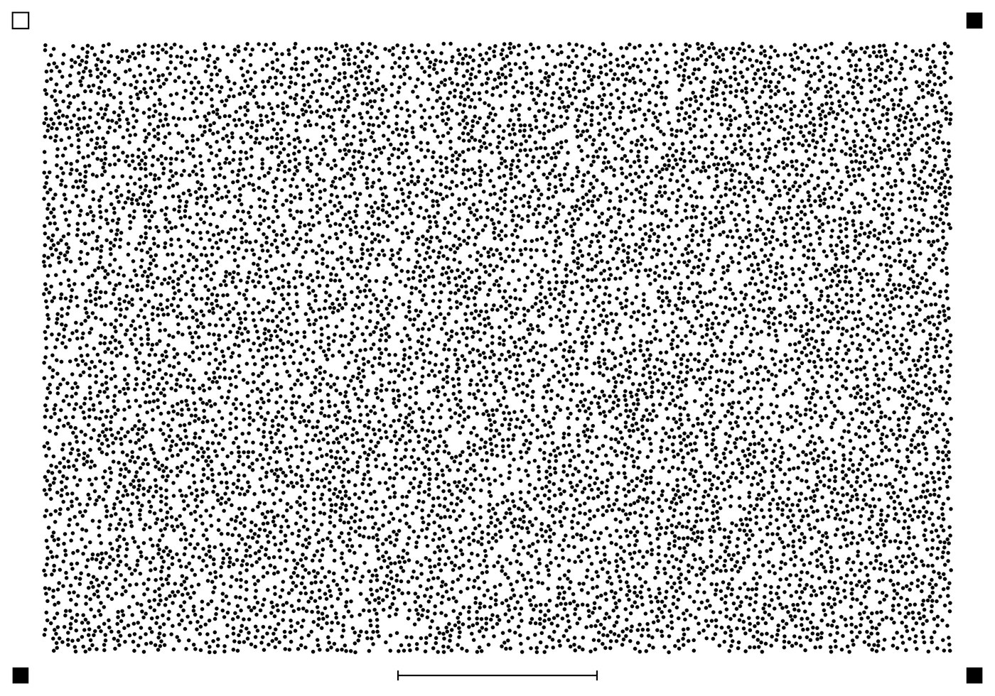
Prototype softwareAn iPhone and Mac app that I built for fun. It turns a phone camera into a background-oriented schlieren (BOS) system. The app generates a random-dot background and captures a reference frame and a flow frame through it. It then cross-correlates the two frames to find the apparent dot displacement that density gradients cause. Examples are the plume above a candle or a heat gun.
WhatSeeing density with a background
Schlieren imaging shows density gradients in a transparent flow. Background-oriented schlieren does this without mirrors or knife edges. A camera photographs a textured background through the flow, and light bent by the gradients shifts the apparent position of the texture. The measured shift gives the deflection. With the geometry, the deflection then gives the gradient.
The Gladstone–Dale relation, the ray deflection through the flow, and the image displacement that it causes for a background distance \(Z_D\) and magnification \(M\).
HowFrom dots to a displacement field
- Generates seeded, reproducible random-dot targets (fine, balanced or coarse) with corner codes for detection.
- Captures a baseline frame and a flow-on frame with focus, exposure and white balance locked, or selects frames from video at up to 240 fps.
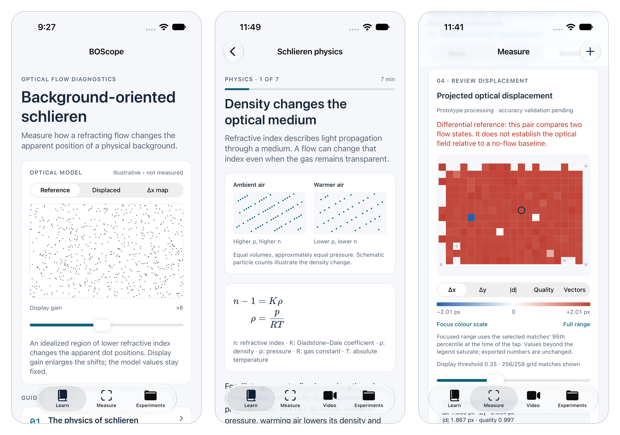
- Estimates a two-component, sub-pixel displacement field by local normalized cross-correlation.
- Shows signed Δx and Δy, magnitude and quality maps, vectors and a grayscale schlieren image.
- Exports everything (images, CSV vectors, JSON metadata) as one archive.
- Optionally uses LiDAR depth to check the distances that set the sensitivity.
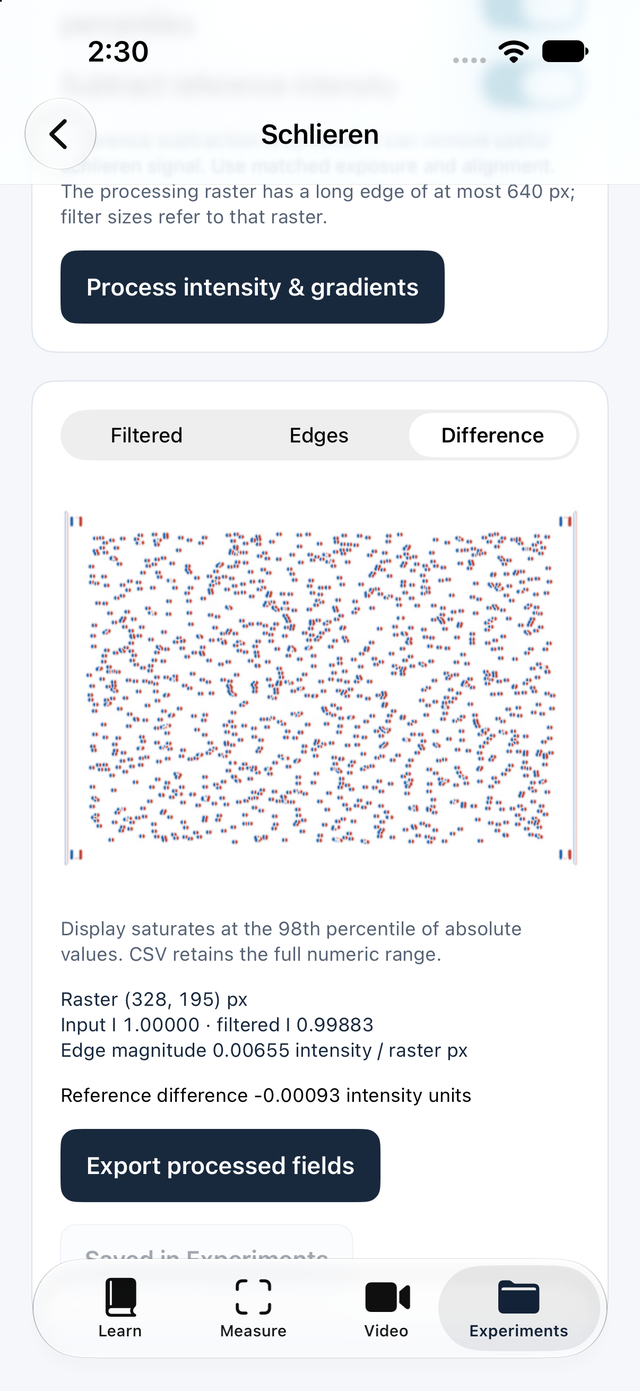
Normalized cross-correlation between interrogation windows of the reference and flow images. The sub-pixel peak gives the local displacement.
ResultsScope of the prototype
The full pipeline runs on the phone: target, capture, correlation, inspection and export. But it does not guarantee accuracy. The synthetic-shift, physical target-motion and ray-angle checks are not complete, so the app labels its results as prototype processing. Density and temperature reconstruction, 3-D reconstruction and velocimetry are not implemented.
The Learn tab is also a short course on schlieren physics. It includes a gallery from the MECH 489 Z-type schlieren lab that started the project.