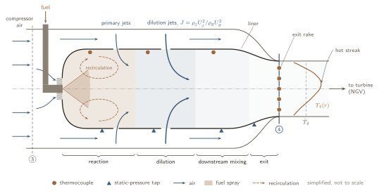
How do fuel properties alter mixing, reaction and heat release, and how do these processes jointly govern combustor turbulence, pollutant formation and the non-uniform flow state delivered to the turbine?
Sustainable aviation fuels can cut life-cycle greenhouse-gas emissions using existing aircraft and fuel infrastructure. Drop-in fuels can still burn differently: differences in composition and physical properties change evaporation, fuel–air mixing, reaction rates and heat release [1, 2].
Full-scale tests show particle reductions with low-aromatic fuels [3, 4], but they do not isolate the mixing and oxidation mechanisms behind them. Soot forms intermittently in fuel-rich regions and can oxidize as mixing proceeds [5]. Mean temperature, pressure and mass flow cannot describe these local processes, or the conditions leaving the combustor.
I measured micro-turbojet performance and emissions [6, 7, 9], and the data supported assessment of collaborators’ engine-performance model coupled to a chemical reactor network [8].
Each of these three areas answers part of the question. Fewer studies follow one fuel effect from the combustor all the way to the turbine inlet. That link is what I want to work on.
How fuel choice changes engine performance or exhaust emissions.
Controlled combustors that resolve local soot formation and oxidation.
[5]
How fuel-dependent combustion, local fuel–air ratio, residence time and combustor flow jointly govern pollutant formation and shape the non-uniform temperature, pressure, composition and flow entering the turbine.
The first part is well established. The open part is the size of the fuel effect on the flow itself. At fixed geometry, matched inlet conditions and matched heat input, I want to measure that effect and find out whether it is large or small.
Emissions or temperature change with fuel, but measured pressure profiles and model-supported flow structure do not.
Reproducible pressure-profile changes, plus model-supported changes in recirculation, dilution mixing or turbulence, beyond experimental and modelling uncertainty.
If the differences stay inside the uncertainty, the question stays open. To link a result to one fuel property, such as volatility or aromatic content, I need more than two fuels.
Each step below is a standard relation. Together they show how one change in the fuel can travel through the whole combustor and into the turbine.
Heat release rate \(\dot q\) along the combustor axis \(x\), hot-gas temperature \(T_g\) and density \(\rho_g\), jet-to-crossflow momentum-flux ratio \(J\), exit temperature field \(T_4\), pattern factor, combustion efficiency \(\eta_c\) and emission indices.
Heat release rate. Volatility decides where the fuel evaporates, and so where it can burn. For a single droplet, the classical \(d^2\)-law gives the evaporation time [18]:
Initial diameter \(d_0\), gas conductivity \(k_g\) and specific heat \(c_{p,g}\), liquid density \(\rho_l\), and the Spalding transfer number \(B\) with gas temperature \(T_\infty\), droplet surface temperature \(T_s\) and latent heat \(h_{fg}\). A less volatile fuel has a lower \(B\). It evaporates more slowly and releases its heat further downstream. Viscosity and surface tension set \(d_0\) through atomization, and \(t_{\mathrm{evap}}\) grows with \(d_0^2\).
Mixing. The dilution jets enter a crossflow whose density is set by the heat released upstream. For the same jets, at a fixed crossflow mass flux \(G_g=\rho_g U_g\) and pressure \(p\), the momentum-flux ratio becomes:
Jet \(j\) and hot crossflow \(g\). Jet penetration \(y\) scales with the jet diameter \(d_j\) and with \(\sqrt{J}\) [17]. A hotter crossflow lowers \(J\), so the jets penetrate less and the mixing pattern moves. This is the route by which chemistry could feed back on large-scale mixing.
Engine performance. The exit temperature field goes into the turbine. Rearranging the pattern factor from step 01 of the plan gives the peak temperature at the turbine inlet. Unburned CO and hydrocarbons set the combustion efficiency [19]:
EI in g per kg of fuel, \(\mathrm{LHV}_{\mathrm{CO}}\approx10.1\) MJ/kg. At the same mean exit temperature, worse mixing raises PF and puts a hotter streak on the first turbine vanes. Illustrative values: with \(\bar T_3=800\) K and \(\bar T_4=1600\) K, PF from 0.20 to 0.25 lifts \(T_{\max}\) from 1760 K to 1800 K.
Pollutants. Thermal NO has a very high activation temperature, so small changes in peak temperature matter. CO burns out only if the gas stays hot long enough [18]:
Initial-rate form of the Zeldovich mechanism, valid while NO is far below equilibrium. The NO formed grows with this rate times the residence time at high temperature. Illustrative values: from 2000 K to 2050 K, \(k_1\) alone rises by about 1.6×. CO burns out where the Damköhler number \(\mathrm{Da}_{\mathrm{CO}}\gg1\). Dilution air that arrives too early quenches the gas and freezes CO.
Soot forms in fuel-rich pockets and burns out in hot gas with oxygen. Both depend on where the mixing puts the fuel and the air. Mixing and residence time appear in every step, so a change in the flow changes all three pollutants.
A large effect would mean fuel studies cannot treat the combustor flow as fixed. A small effect would mean the flow can be taken from one fuel and reused, which makes modeling much cheaper.
Peak-to-mean excess over the combustor temperature rise.
Step 3 stops at the simplest rung that preserves measured exit-profile shapes and fuel-dependent differences within uncertainty.
Global equivalence ratio, pattern factor, and a combined standard uncertainty from the systematic part \(b\) and the scatter \(s\) of \(n\) repeats, expanded with coverage factor \(k\approx2\).
Favre-averaged (density-weighted) RANS balances for mass, momentum and species \(k\).
Boussinesq closure of the Reynolds stresses, heat release from the species sources, and residence time of a region of volume \(V\) carrying mass flow \(\dot m\). Withheld spatial measurements decide whether an explanation holds.
Mass-weighted mean and non-uniformity of the exit temperature, turbulence intensity, and the model-derived turbulence length scale (\(C_\mu=0.09\)).
The inlet-description ladder, with flow angles \(\boldsymbol\alpha\). Each description is computed from the one before it. Step 3 keeps the simplest description that reproduces measured exit-profile shapes and the supported fuel-dependent differences within uncertainty.
I have not done this work yet. These notes come from a lot of reading and thinking. It is the direction I most want to explore, and I would need guidance to get it right. Items marked Open question are the ones I am least sure about.
| Quantity | Why the turbine cares | How it could be measured |
|---|---|---|
| Exit temperature field, pattern factor | Hot streaks set the vane metal temperature | Traversing thermocouple rake |
| Turbulence intensity \(Tu\), integral length scale \(\ell\) | They drive the extra loss of combustor turbulence [11, 12] | Time-resolved PIV and LDV, which need optical access [20, 21] |
| Swirl and flow angle Open question | Vane incidence and loading | Stereo PIV, or a cooled multi-hole probe where it fits |
| Where heat is released | Where a fuel effect enters the flow | OH* chemiluminescence, OH-PLIF [23] |
| Soot inside the flame | Radiation to the liner | Laser-induced incandescence [22] |
These are qualitative links, using the relations in the panel above and our own fuel tests.
My working guess is that the exit temperature profile and radiation are stronger fuel levers than turbulence. That is a hypothesis.
Which platform, or which combination, is the right one is the first thing I would want to work out with a supervisor.
Linking pollutant formation and the non-uniform turbine-inlet flow through their shared fuel-dependent physics could give a baseline for passing experimentally constrained flow information between combustor and turbine models.
If mixing leaves no detectable fuel-dependent spatial differences, shared temperature or pressure profiles may represent the exit state without being uniform. If it does, the work identifies which spatial quantities to retain, since they may affect turbine loss and heat transfer [11–13].
The baseline could support later high-fidelity simulation [14, 15], turbine-response calculations, and larger-engine comparisons with collaborator models and data; none is required for the PhD.
Low-volume tests support screening and model development. Differences in pressure ratio, geometry, cooling, efficiency and residence time rule out assuming scale equivalence.