P200-SX Exhaust Jet Model & Duct Design

View down the installed exhaust duct from the engine nozzle, with the sampling-probe holder in the foreground

Modeled centerline decay of velocity, temperature and density downstream of the nozzle

The digital twin of the test cell, with the exhaust route from the engine stand to the roof exhaust fan

P200-SX Exhaust Jet Model & Duct Design

Graduate research

This project takes a hot, fast jet out of a closed test cell, safely and without disturbing the engine. A MATLAB model of the free jet sized the ducting. A first concept failed because it set off the CO alarm. The installed duct carries the exhaust upward. The latest design work is a digital twin of the cell.

Result

The model predicted about 18 m/s and 360 K on the centerline 5 m downstream. These are model values. Supports and probe mounts built in-house saved 29% on hardware.

Methods & tools

Self-similar jet model in MATLAB · 0D flow estimates · SolidWorks and Autodesk Fusion · in-house fabrication · 2D RANS (k–ω) in ANSYS Fluent

Project breakdown

WhatWhat the exhaust has to do

The P200-SX sends a hot, high-speed jet into a closed room. The ducting has to:

carry the jet out of the building without back-pressuring the nozzle
entrain enough room air to cool and dilute the jet
leave space for the sampling probe
fit inside an existing cell.

To size the duct, I needed a quantitative picture of how the jet slows, cools and spreads, before any hardware or CFD.

How1 · A marching model of the free jet

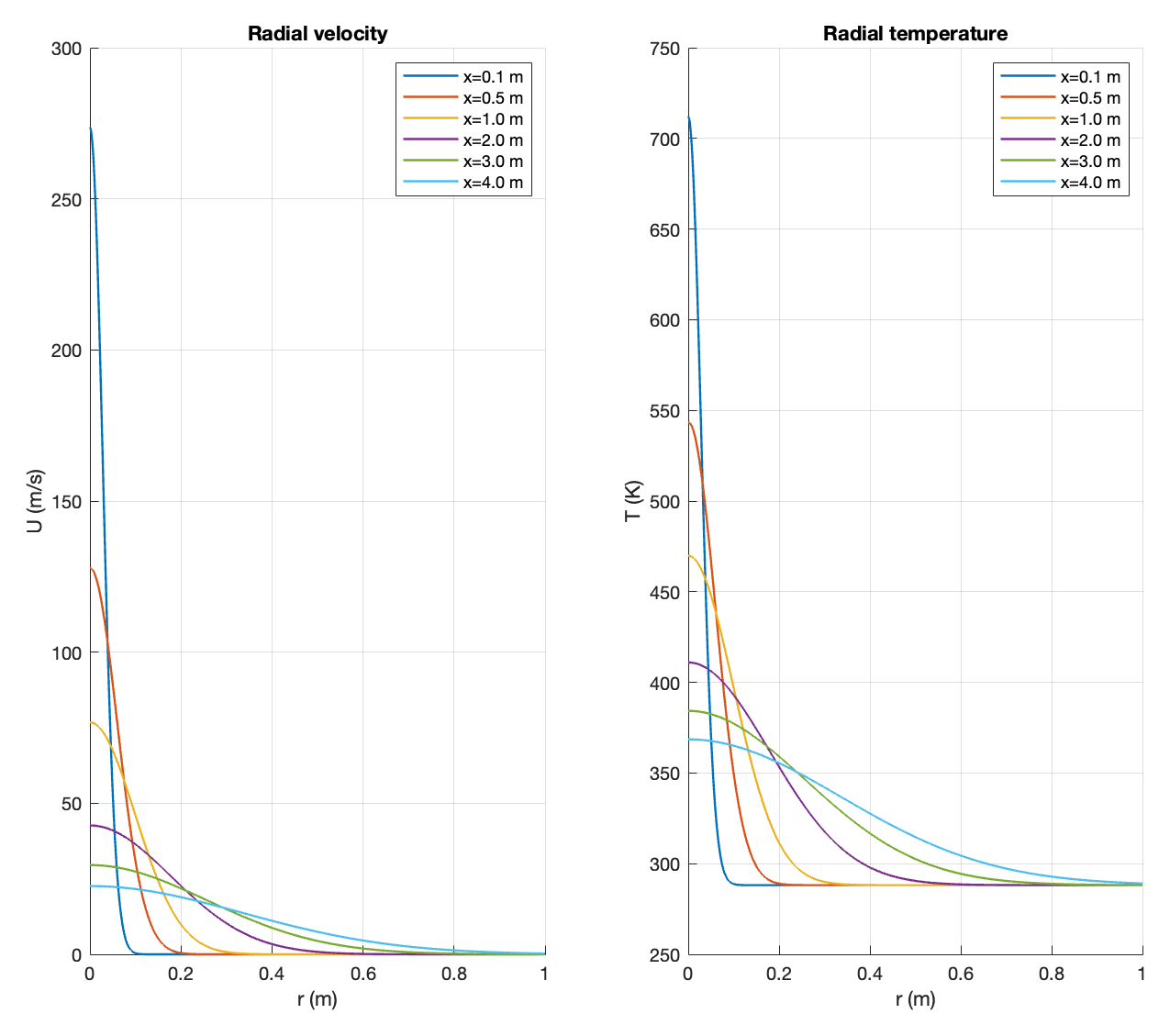
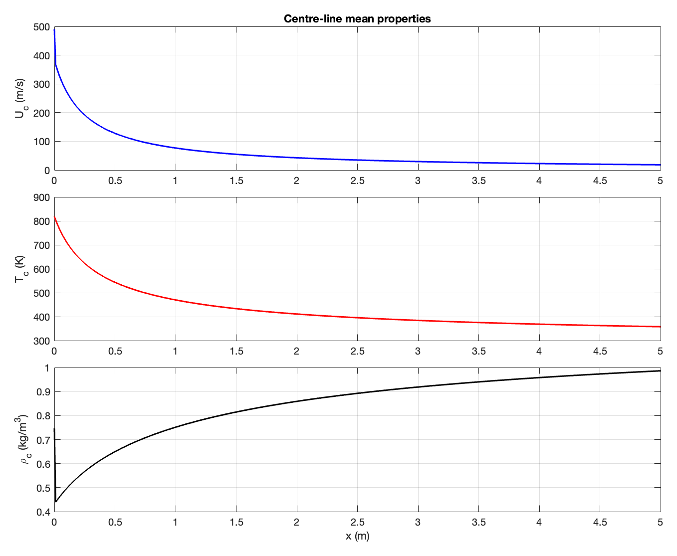
Fig. 1 — Self-similar radial profiles of velocity and temperature at stations downstream of the nozzle.

I modeled the exhaust as a free, axisymmetric turbulent jet in still air. A MATLAB marching model steps downstream from the nozzle. It uses Gaussian self-similar profiles, momentum and enthalpy conservation, a linear spreading rate and an eddy-viscosity closure, with constants from the turbulent-jet literature. The Method view in the gallery above shows the centerline decay.

\[\frac{U(x,r)}{U_c(x)}=\exp\!\left[-\left(\frac{r}{b(x)}\right)^{2}\right],\qquad \frac{U_c}{U_j}=\frac{B\,d}{x-x_0},\qquad b=S\,(x-x_0)\]

Gaussian self-similar profile with half-width \(b(x)\), inverse centerline decay with constant \(B\) from the virtual origin \(x_0\), and linear spreading at rate \(S\). Temperature follows the same similarity, with enthalpy conservation.

The physics is simple. The momentum flux is conserved, so as the jet entrains still air, its width grows linearly and its centerline velocity falls as \(1/x\). I checked the decay trends against 0D estimates for both the velocity field and the thermal field.

≈ 18 m/scenterline velocity 5 m downstream

≈ 360 Kcenterline temperature at 5 m (adiabatic mixing)

29%hardware cost saved by in-house fabrication

Five meters downstream, the centerline has slowed to about 18 m/s and cooled to about 360 K. This prediction set the duct diameters. It also suggested that entrainment could supply the dilution the sampling system needs. The same geometry then became the domain for a 2D k–ω RANS model in ANSYS Fluent. That model gave a second estimate of the jet evolution and the flow uniformity in the duct.

How2 · The first concept, and why it was dropped

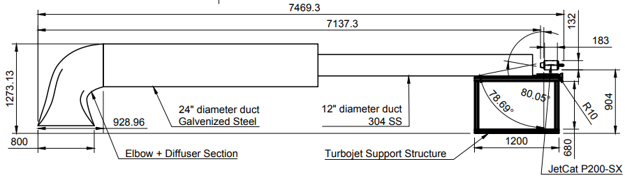
Early concept, not built: a 12-inch stainless elbow and diffuser stepping up to a 24-inch galvanized outlet, about 7.5 m overall. — Fig. 2 — **Early concept, not built:** a 12-inch stainless elbow and diffuser stepping up to a 24-inch galvanized outlet, about 7.5 m overall.

The first design, done in SolidWorks, was a dual duct that turned the exhaust down and away from the engine. Two problems ended it. First, in-house fabrication of the elbow and diffuser proved impractical. Second, a test of a simplified elbow showed that the turn itself was at fault. Directing the exhaust toward the floor caused enough recirculation to set off the test cell’s CO alarm. A duct that looks reasonable on paper can still return exhaust to the room.

How3 · The duct as installed

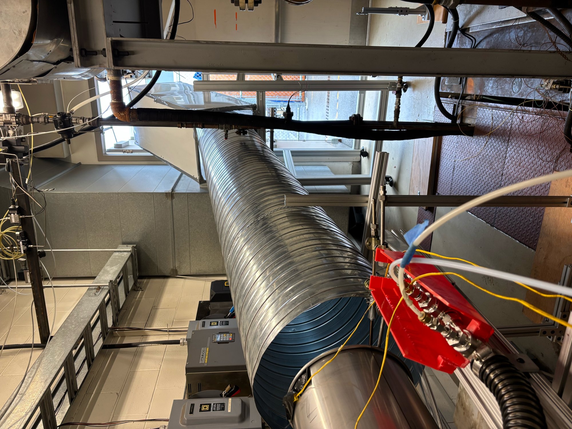
The installed duct deflects the exhaust about 30° upward into a straight run, away from the floor. A 12-inch section extended it in December 2025. The supports and probe mounts were built in-house from repurposed stock.

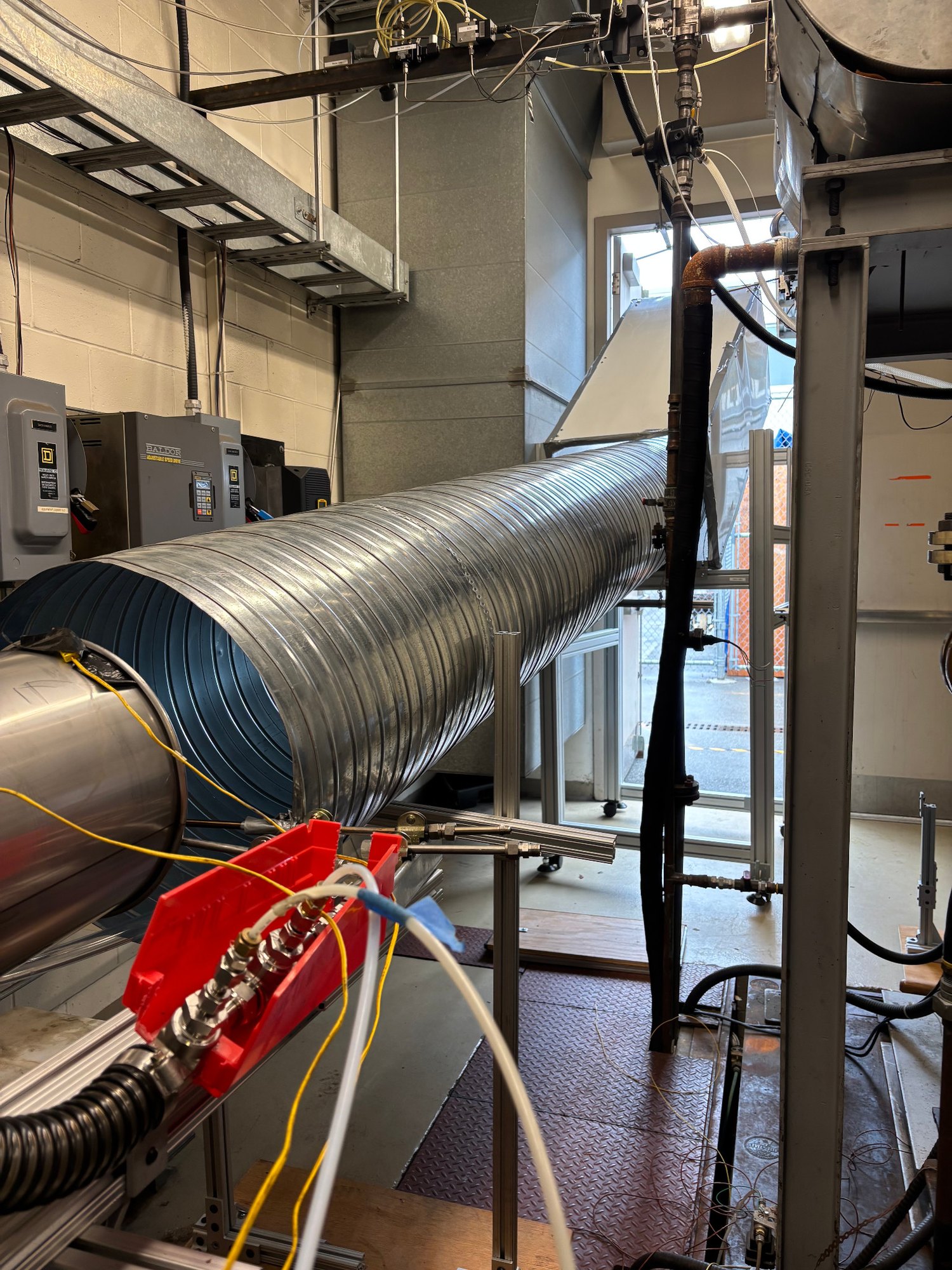
Fig. 3 — The installed duct with thermocouples on the sampling probe.

The exhaust is also sampled in the duct. The probe holder, thermocouples and lines are therefore part of the design from the start.

Results4 · A digital twin of the cell

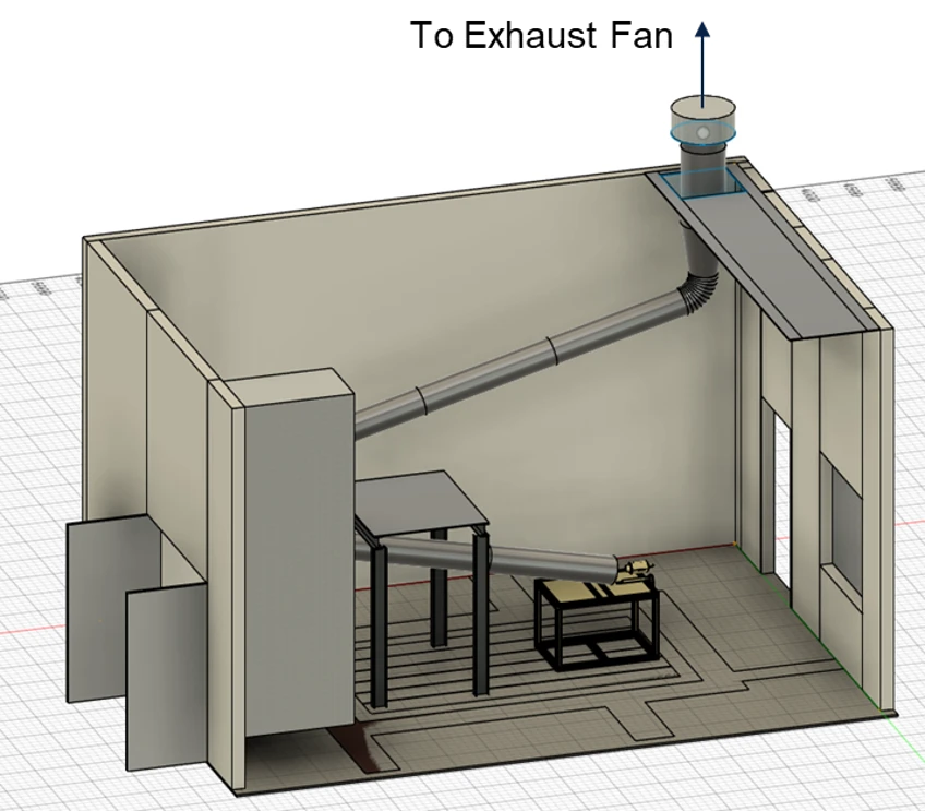
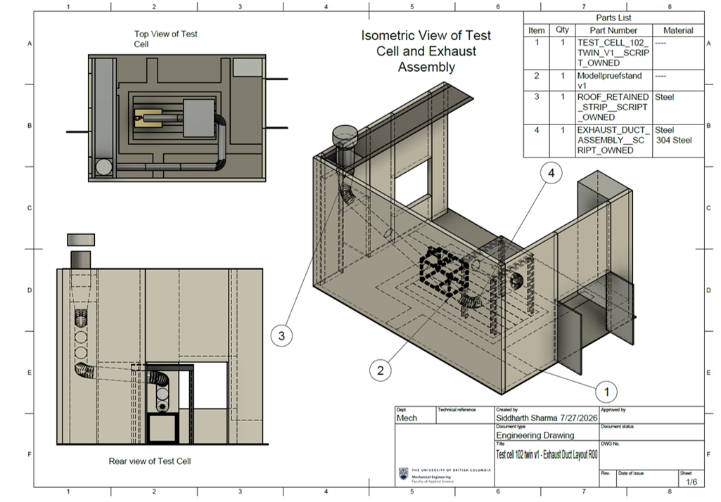
The latest design work is a digital twin of the whole test cell, shown as the Result view at the top. It is a CAD model of the walls, the engine stand, the roof-retained strip and the steel duct assembly. With it, a new route or a second engine can be checked against the real geometry before anything is cut. The layout drawing below is its first release (R00, July 2026).

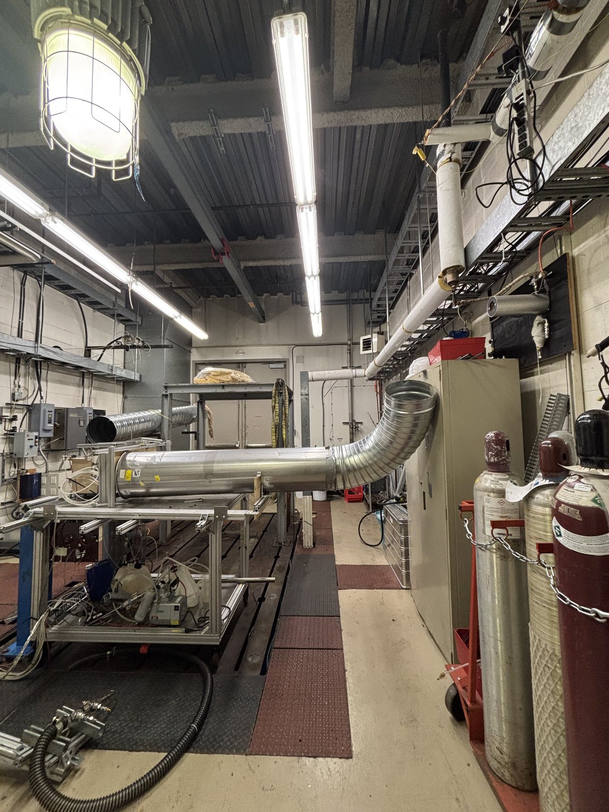
Fig. 4 — Exhaust-duct layout drawing for the test-cell digital twin (Test cell 102 twin v1, R00, July 2026), with top, rear and isometric views and the parts list.

Fig. 5 — Newer setup work in the test cell: exploring layout options with the ducting and supplies we already have.

The newest setup work happens in the cell itself. I test layout options with the ducting and supplies we already have, and check them against the twin.