Apollo Ascent Engine Nozzle: A Staged-Fidelity CFD Hierarchy

Home / Projects / Independent computational studies

The exhaust leaves the nozzle at sea-level start-up. A transported mixture fraction tracks nozzle gas (red) as it pushes into still air (blue)

One effect at a time: design-point Mach number for Cases 01–04 (inviscid, + temperature-dependent heat capacity, + viscosity, + SST turbulence). Each panel has its own color scale

The same vacuum nozzle against a sea-level back pressure (101 kPa), so the flow is strongly over-expanded. The inviscid cases show a single normal shock. With viscosity, the flow separates from the wall and a shock train forms

Apollo Ascent Engine Nozzle: A Staged-Fidelity CFD Hierarchy

Independent computational study

A personal project to build rocket-nozzle CFD from the ground up. The test bed is the chamber and bell nozzle of the Apollo Lunar Module ascent engine. Each simulation adds exactly one piece of physics to the last. The sequence is 1-D theory, inviscid flow, a thermally perfect gas, viscous flow, turbulent flow and finally the plume. This shows me what each layer of fidelity actually buys. It also shows, very visually, how a nozzle designed for vacuum over-expands and separates against sea-level back pressure.

Scope

The ascent engine supplies the nozzle geometry and the nominal chamber pressure. Real Aerozine-50/N₂O₄ chemistry is out of scope by design. I did not derive or use a kinetic mechanism for it, or for any other hypergolic propellant. A generic, non-reacting CH₄/O₂ surrogate with Cantera properties stands in for the real propellants throughout. Nothing here is compared with Apollo flight data.

Methods & tools

OpenFOAM v2306 (rhoCentralFoam, Kurganov–Tadmor fluxes) · independent quasi-1-D solver in Python · Cantera property fits · k–ω SST · passive scalar transport · ParaView post-processing on WSL2

Project breakdown

WhatWhy build it one layer at a time

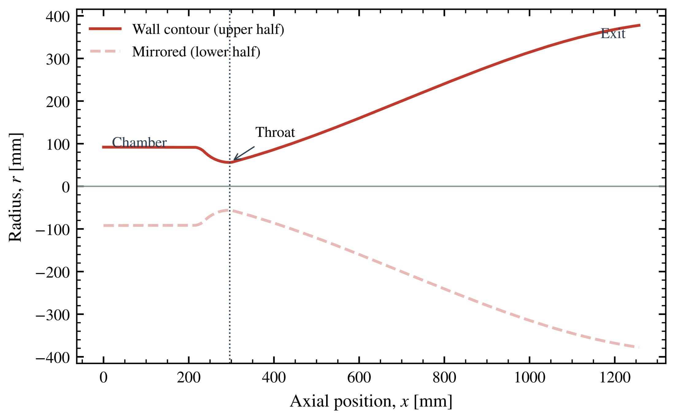
High-fidelity rocket CFD fails in ways that are hard to diagnose when all physical effects are active at once. I went the other way. I start from a model that I can check by hand and add one effect per case. I explain every change in the answer before I move on. The ascent engine is a good test bed because its geometry is well documented. It has a 91.9 mm chamber radius, a 55.9 mm throat and a 377.7 mm exit, an area ratio of 45.6 over 1.26 m [1].

Fig. 1 — Nozzle contour from the reference geometry: chamber, throat and a long bell to an exit area 45.6 times the throat area.

Real Aerozine-50/N₂O₄ chemistry is out of scope by design. I did not derive or use a kinetic mechanism for it, or for any other hypergolic propellant. A generic, non-reacting CH₄/O₂ surrogate stands in for the real propellants throughout. Its chamber state is a Cantera equilibrium at O/F 3.5, about 3,334 K and the nominal 0.848 MPa of the engine. The composition then stays frozen through the nozzle [9]. This keeps the fluid dynamics honest, but the thrust and specific impulse are not Apollo numbers.

The hierarchy: one physical effect per case
Case	What it adds	Cells
00	Independent quasi-1-D isentropic solver along the contour	1-D
01	2-D axisymmetric, inviscid, constant heat capacity (γ = 1.209)	10,000
02	Temperature-dependent heat capacity (NASA-7 fit, frozen composition)	10,000
03	Viscosity and a no-slip wall (laminar), first cell sized for y⁺ ≈ 1	16,800
04	k–ω SST turbulence with a low-Re wall treatment	16,800
05	External plume domain with a transported mixture fraction	36,900

Like the Sandia work, this runs on my gaming laptop. The hardware and its limits are on the Sandia Flame D page. A fine nozzle-and-plume domain does not fit in it. I build the case in steps and keep each mesh as small as the physics allows. Annoying, but it forces good case design.

HowThe physics in each layer

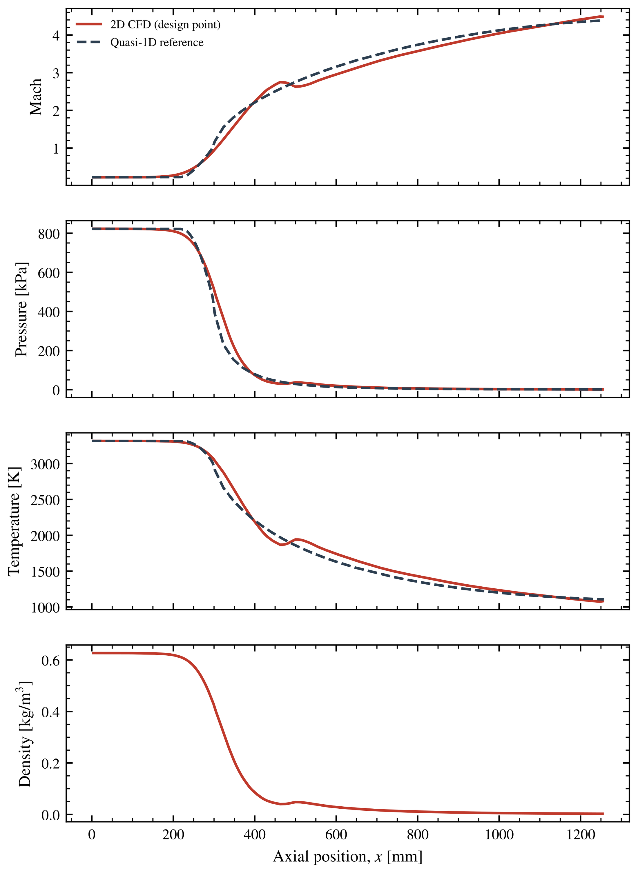
The 2-D cases use rhoCentralFoam, the density-based, shock-capturing solver in OpenFOAM, with Kurganov–Tadmor central-upwind fluxes [4, 5]. Case 00 is the textbook reference. It inverts the area–Mach relation along the contour, then computes thrust from the exit plane. That thrust includes the pressure term, which becomes the whole story off design [2, 3]:

\[\frac{A}{A^*}=\frac{1}{M}\left[\frac{2}{\gamma+1}\left(1+\frac{\gamma-1}{2}M^2\right)\right]^{\frac{\gamma+1}{2(\gamma-1)}},\qquad F=\dot m\,u_e+\left(p_e-p_a\right)A_e,\qquad I_{sp}=\frac{F}{\dot m\,g_0}\]

The area–Mach relation, thrust with the pressure term \((p_e-p_a)A_e\), and specific impulse. At \(\gamma=1.209\), an area ratio of 45.6 gives an exit Mach number of 4.39.

Fig. 2 — Case 01 centerline compared with the independent quasi-1-D solution: Mach number, pressure, temperature and density along the nozzle. The small bump near x ≈ 0.47 m is a 2-D recompression that 1-D theory cannot see.

Then the physics goes in. Case 02 lets the heat capacity follow temperature, so the local γ changes through the nozzle. Case 03 adds viscosity with a Sutherland fit and a no-slip wall. Its mesh puts the first cell at y⁺ below 1. Case 04 adds the SST model of Menter. Its limiter keeps the eddy viscosity bounded through the strong gradients at the throat [6]:

\[\mu(T)=\frac{A_s\sqrt T}{1+T_s/T},\qquad \nu_t=\frac{a_1k}{\max(a_1\omega,\;SF_2)},\qquad y^+=\frac{\rho_wu_\tau y_1}{\mu_w}\]

Sutherland viscosity, the SST eddy-viscosity limiter and the wall coordinate used to size the first cell.

The boundaries took the most effort. A plain zero-gradient outlet crashed five consecutive starts, and a non-reflecting outlet fixed that. A second bug was a sustained acoustic resonance. It came from a relaxation length that I copied from a 30 mm tutorial, and rescaling that length to this domain cured it [7].

ResultsWhat each layer of fidelity buys

Design point (1,449 Pa back pressure). *Specific impulse is derived from thrust and mass flow. The gas is a surrogate, so these are not Apollo values. There is no grid-convergence study, so differences of about 1% are not shown to exceed the discretization error
Case	Exit T	Exit p	Exit speed	Vacuum thrust	I_sp,vac*	Mass imbalance
00 quasi-1-D	1,107 K	1,444 Pa	3,192 m/s	15,709 N	339.5 s	—
01 inviscid	1,129 K	1,728 Pa	3,171 m/s	15,342 N	333.4 s	0.05%
02 + C_p(T)	972 K	1,527 Pa	3,148 m/s	15,150 N	329.0 s	0.003%
03 + viscosity	1,010 K	1,611 Pa	3,115 m/s	15,010 N	327.1 s	0.16%
04 + SST	1,021 K	1,540 Pa	3,112 m/s	14,890 N	326.0 s	0.05%

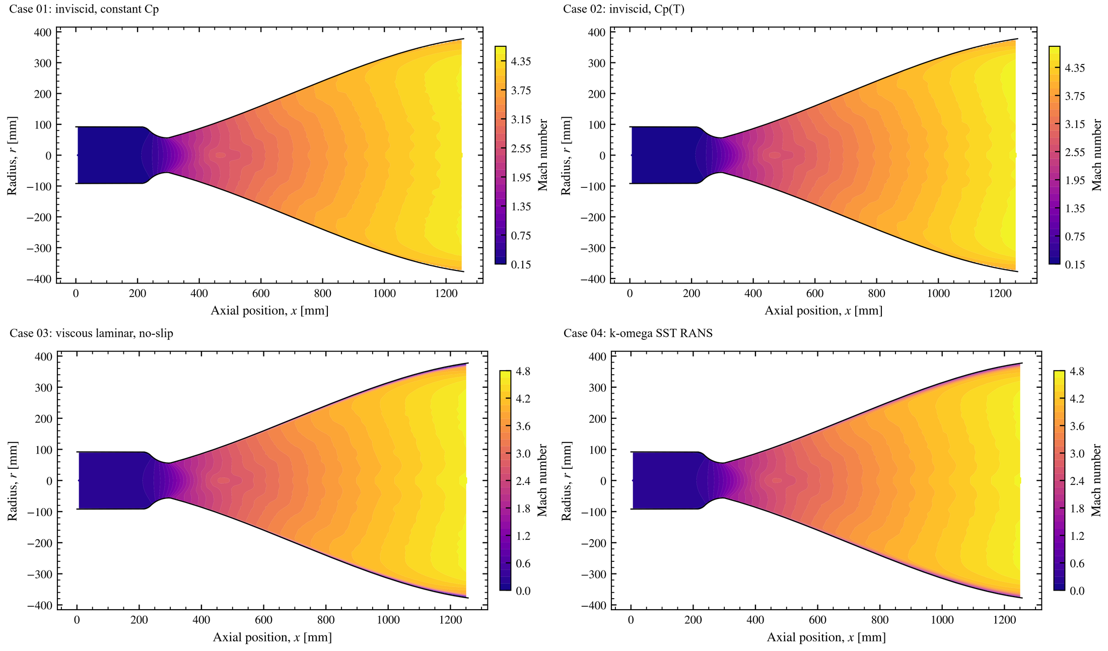
2-D vs 1-D (Case 01): the exit speed agrees within 0.7%, but thrust drops 2.3%. The main reason is that 2-D flow leaves the bell with a radial velocity component (about 647 m/s), which 1-D theory ignores.
Temperature-dependent heat capacity (Case 02): the biggest change in the temperature field (the exit is 14% cooler), but only 1.3% in thrust. Most of the energy is already kinetic by the exit.
Viscosity (Case 03): a thin, hot boundary layer and wall friction cost another 0.9% of thrust. The core flow barely moves.
Turbulence (Case 04): modeled turbulent stresses make the layer slightly thicker (−0.8%). On the centerline the solution is almost unchanged.

Fig. 3 — Design-point temperature for Cases 01–04 (each with its own color scale). Temperature-dependent heat capacity gives a cooler expanding core, and the no-slip cases add a hot layer along the wall.

Fig. 4 — Case 02: the local ratio of specific heats, from about 1.21 in the hot chamber to 1.29 in the cold exit flow.

Fig. 5 — Wall y⁺ for Cases 03 and 04 is below 1 everywhere (maximum 0.81 and 0.91). The equations are integrated all the way down to the wall, with no wall function. In Case 04 the SST model still models the turbulent stresses.

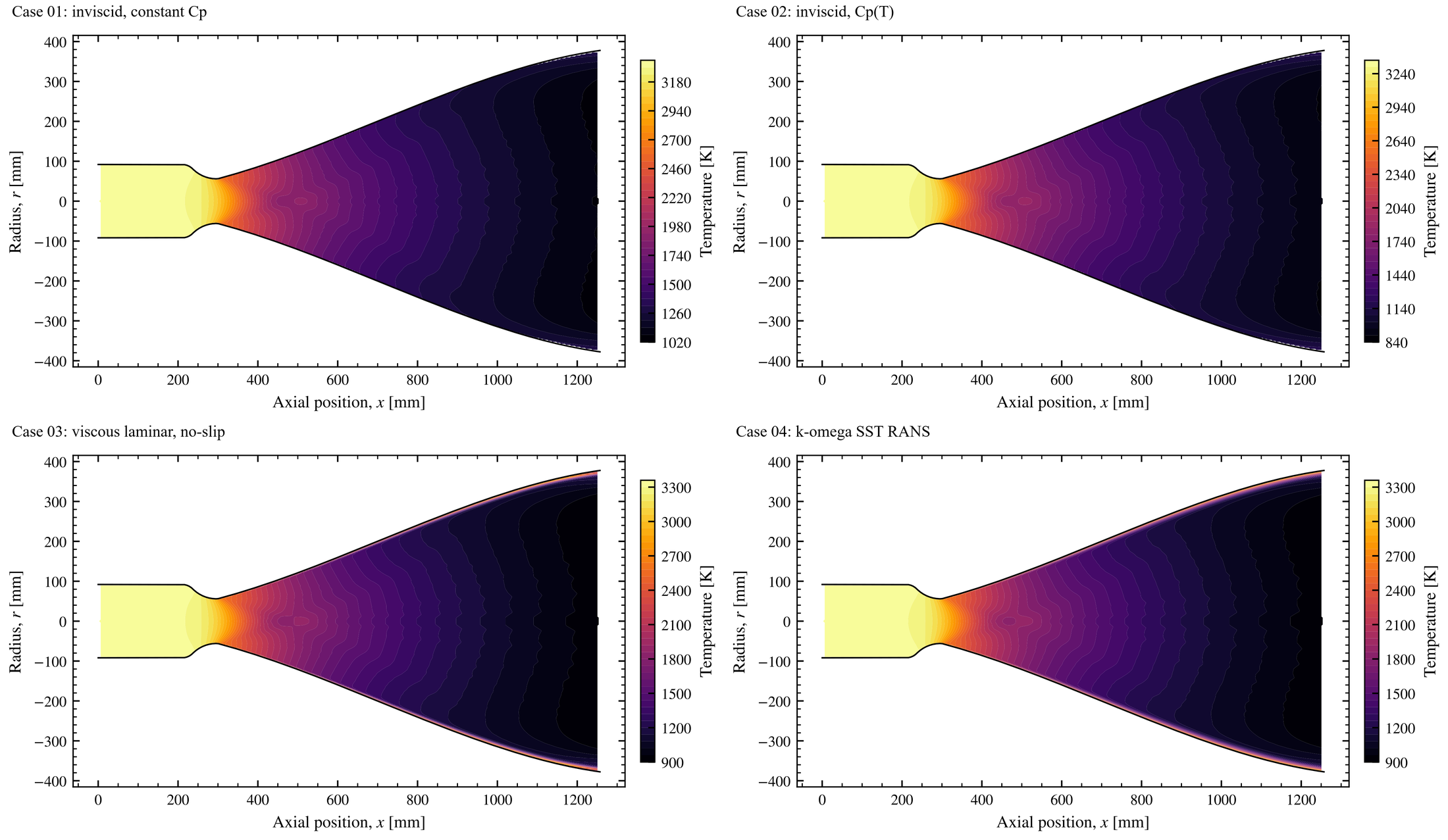
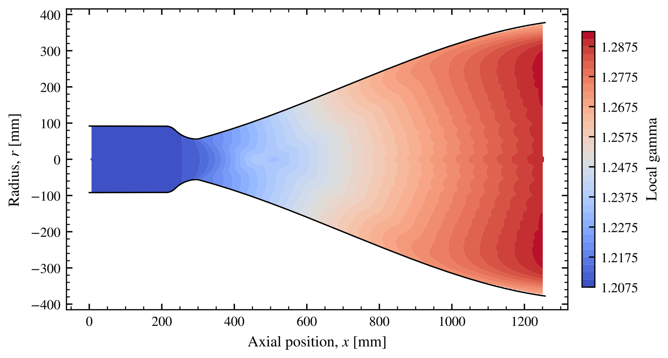
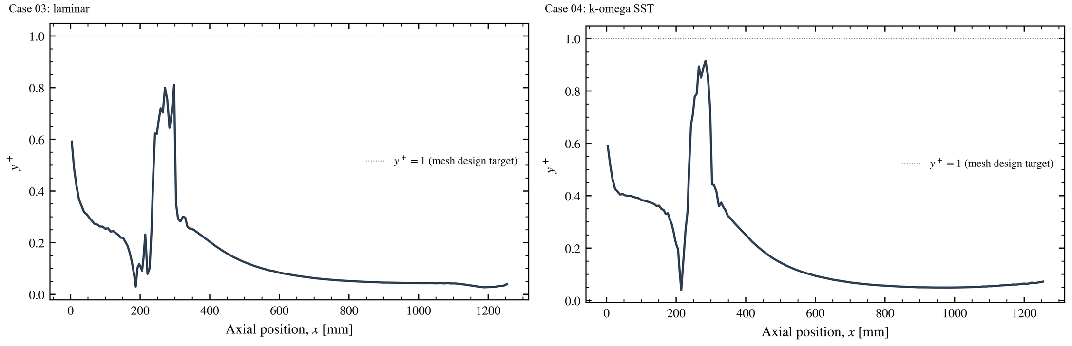
The pattern is the useful lesson. Each extra layer of physics changes the thrust by about 1%, but it changes what you can see in the flow far more. There is no grid-convergence study, so I cannot show that differences this small are larger than the discretization error. If the question is performance, the inviscid model with temperature-dependent heat capacity gets most of the way. If the question is heat load or separation, the wall physics is everything. Every step is internally consistent and conserves mass to better than 0.16%.

ResultsVacuum nozzles vs sea-level nozzles

A nozzle gives the most thrust when its exit pressure matches the surrounding pressure. That is why engines are built for where they fire. A sea-level engine has a much shorter nozzle (area ratios typically of order 10–20), so its exit pressure stays near one atmosphere. A vacuum engine like the ascent engine uses a long, wide bell (an area ratio of 45.6 here) to continue to expand the gas. This turns more of its enthalpy into exhaust velocity [2]. Run either one away from its design pressure and energy is wasted.

\[F=\underbrace{\dot m\,u_e}_{\text{momentum}}+\underbrace{\left(p_e-p_a\right)A_e}_{\text{pressure mismatch}},\qquad \nu(M)=\sqrt{\frac{\gamma+1}{\gamma-1}}\tan^{-1}\!\sqrt{\frac{\gamma-1}{\gamma+1}\left(M^2-1\right)}-\tan^{-1}\!\sqrt{M^2-1}\]

Thrust is maximized when \(p_e=p_a\). If \(p_e>p_a\), the flow is under-expanded. It continues to turn outward through expansion fans (Prandtl–Meyer function \(\nu(M)\)) after it leaves. If \(p_e\ll p_a\), the flow is over-expanded and the atmosphere pushes back through shocks.

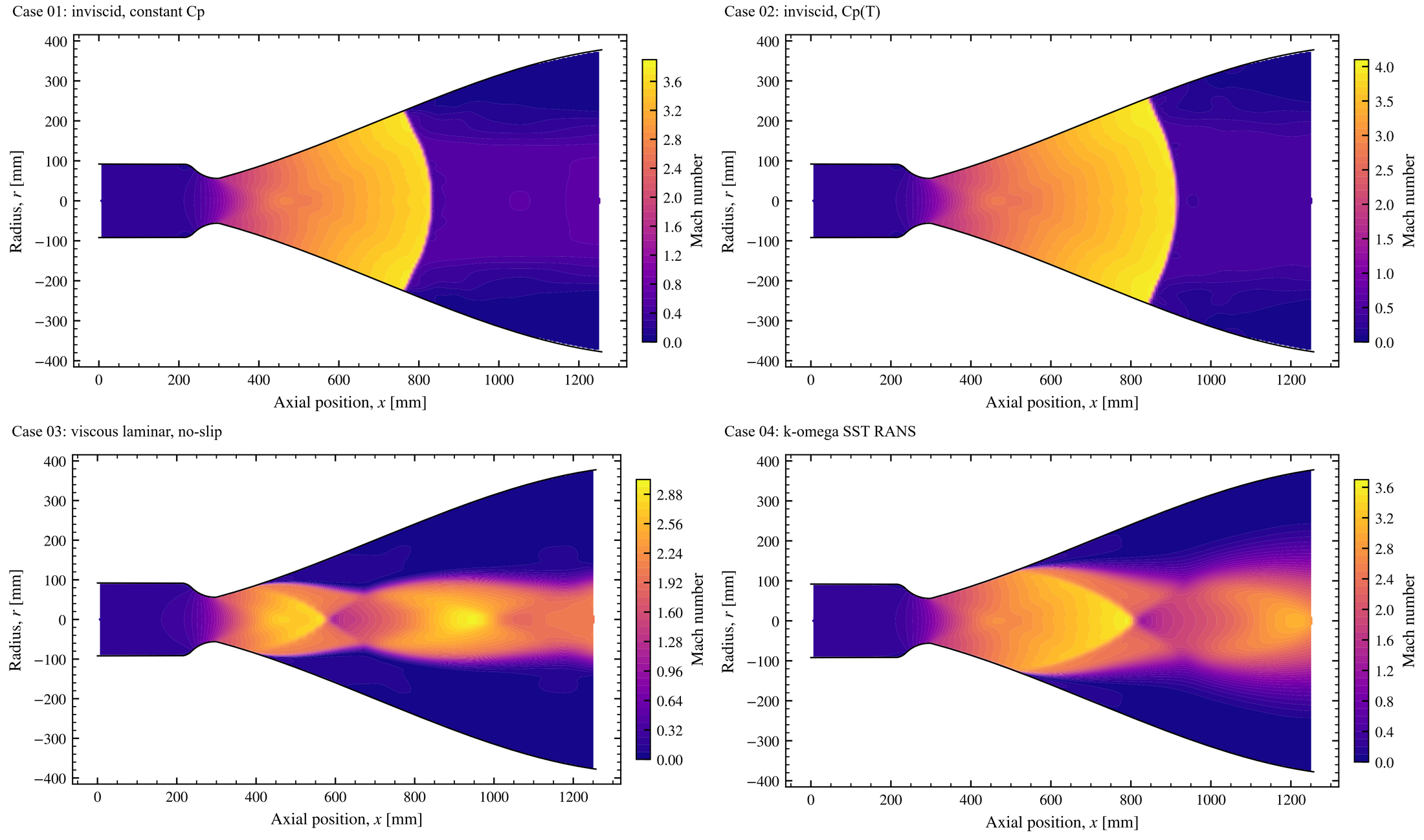
To reach the design point, I used a back-pressure ladder that lowers the outlet pressure in steps from 101 kPa to 1.45 kPa. The ladder is only a numerical path to the design point. Its first rung is sea-level back pressure. I plotted the sea-level cases on purpose, to show the over-expansion and the shocks it drives into the bell. I think the shocks and the throat expansion look cool as hell.

Fig. 6 — Case 01 Mach number at sea level (top, 101 kPa) and at the design point (bottom, 1.45 kPa). At sea level, a near-normal shock stands inside the bell and all the flow after it is subsonic.

Fig. 7 — The same two cases as numerical schlieren (density-gradient magnitude). The expansion fan comes off the throat curvature, and at sea level a curved shock crosses the bell.

Fig. 8 — Sea level, all four fidelity levels as numerical schlieren. The inviscid cases hold one curved normal shock. With viscosity, the boundary layer cannot climb the pressure rise and the flow separates from the wall. Oblique shocks then cross into a Mach disc and a train of shock cells. The viscous panels are not mass-converged at this leg.

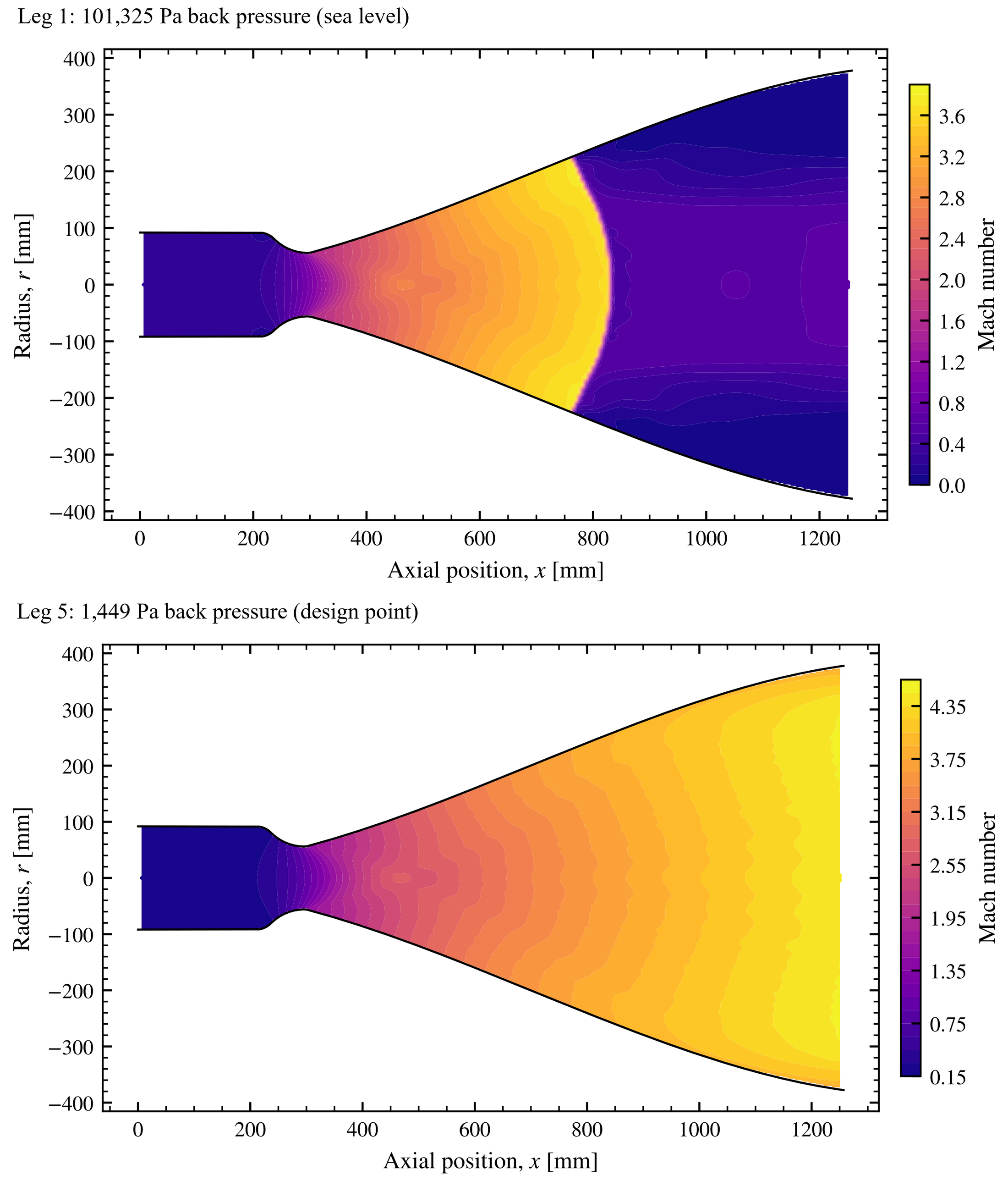
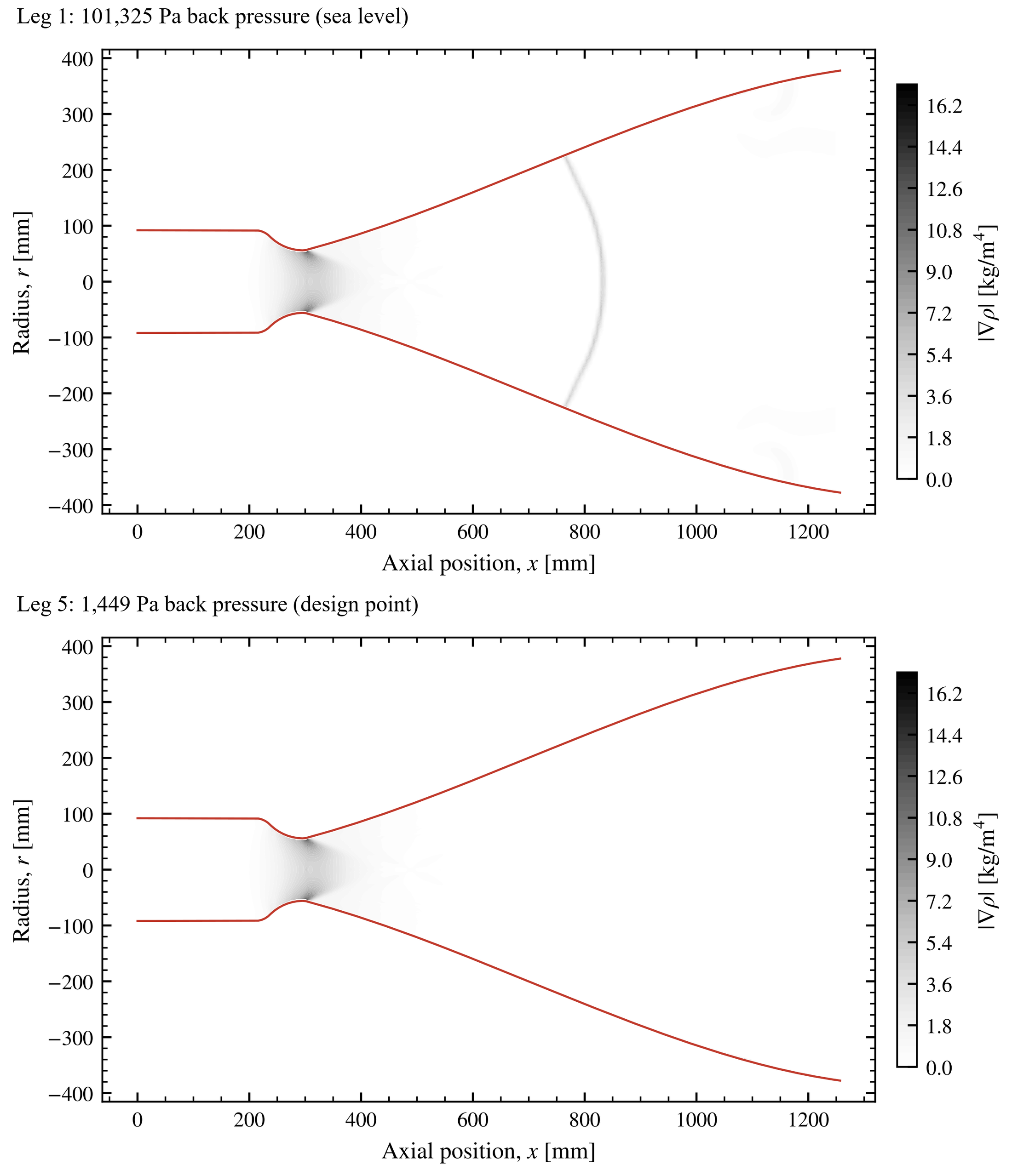
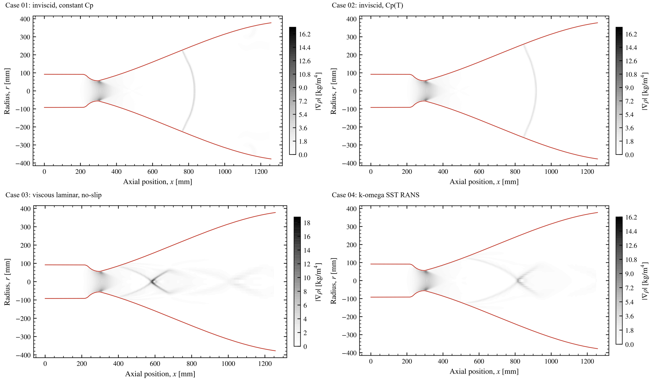
At sea level, the exit pressure of this nozzle would be about 1.7% of atmospheric pressure, so the flow is wildly over-expanded. The inviscid models answer with a single normal shock that stands in the bell. Viscosity changes the picture completely. The slow boundary layer cannot climb that pressure rise, so the jet separates from the wall. Oblique shocks then cross into a Mach disc and a chain of shock cells.

Against sea-level back pressure, this vacuum nozzle runs strongly over-expanded, with internal shocks and, in the viscous cases, separation. In this study, sea level is only the first rung of the numerical ladder. The viscous sea-level fields are not mass-converged, so I use them for the flow structure only.

Estimated thrust of the Case 01 nozzle, \(F=F_{vac}-p_aA_e\) with \(A_e=0.448\) m². This is a textbook estimate from the design-point solution. At sea level the estimate goes negative. That is unphysical, because a real nozzle separates first, which limits the loss
Ambient pressure	Ideal thrust	Change	I_sp
1,449 Pa (design leg)	14,693 N	−4.2%	319 s
2.5 kPa	14,222 N	−7.3%	309 s
8 kPa	11,757 N	−23%	256 s
30 kPa	1,899 N	−88%	41 s
101.3 kPa (sea level)	negative	—	—

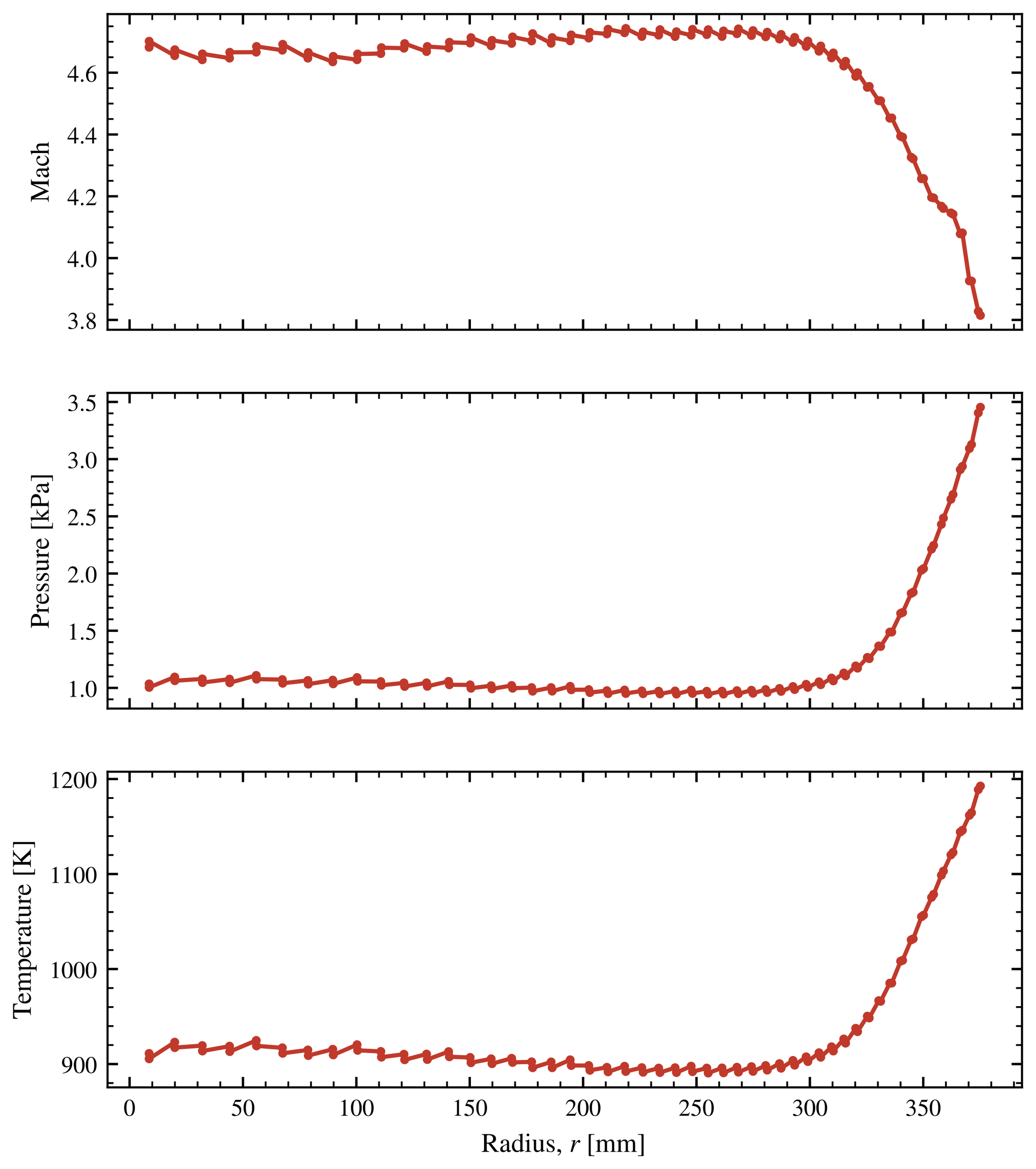
The table puts the wasted energy in numbers. Even at its own design point, the solution is slightly under-expanded. The exit pressure rises from about 1.0 kPa on the axis to 3.4 kPa at the lip, which is above the 1.45 kPa outside. The gas therefore continues to expand through fans that start at the lip, just outside the computed domain. Toward sea level, the pressure term swamps everything.

Fig. 9 — Exit-plane profiles at the design point (Case 02). The Mach number falls from about 4.7 on the axis to 3.8 at the lip, while pressure and temperature rise toward the wall.

ResultsInto the plume

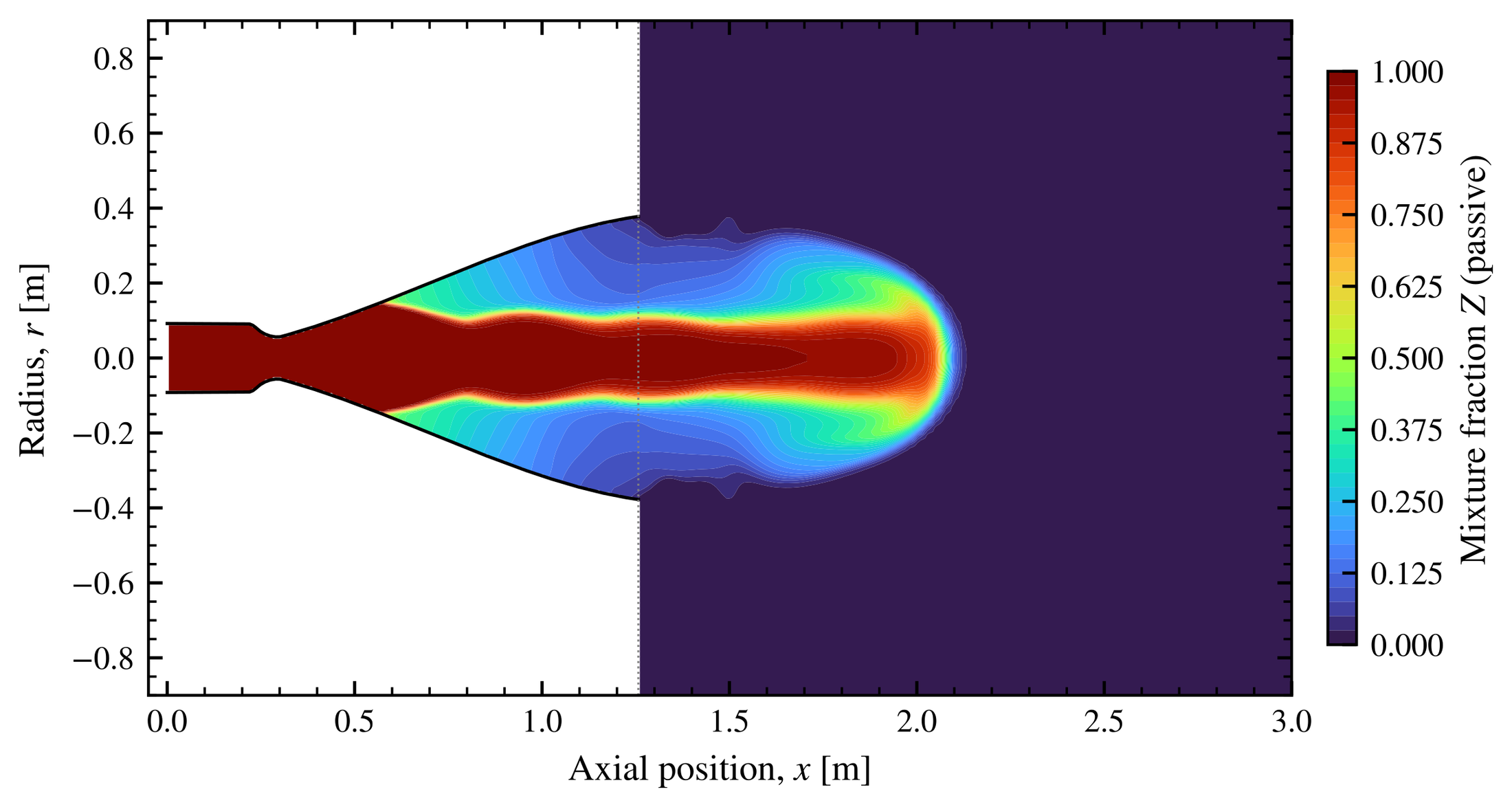
Case 05 extends the domain ten exit diameters downstream and six radially. It transports a passive mixture fraction from the nozzle into the surrounding air [8]:

\[\frac{\partial(\rho Z)}{\partial t}+\nabla\cdot(\rho\mathbf UZ)=\nabla\cdot\big((\mu+\mu_t)\nabla Z\big)\]

Bounded passive-scalar transport with a turbulent Schmidt number of one. \(Z=1\) is nozzle gas and \(Z=0\) is ambient air.

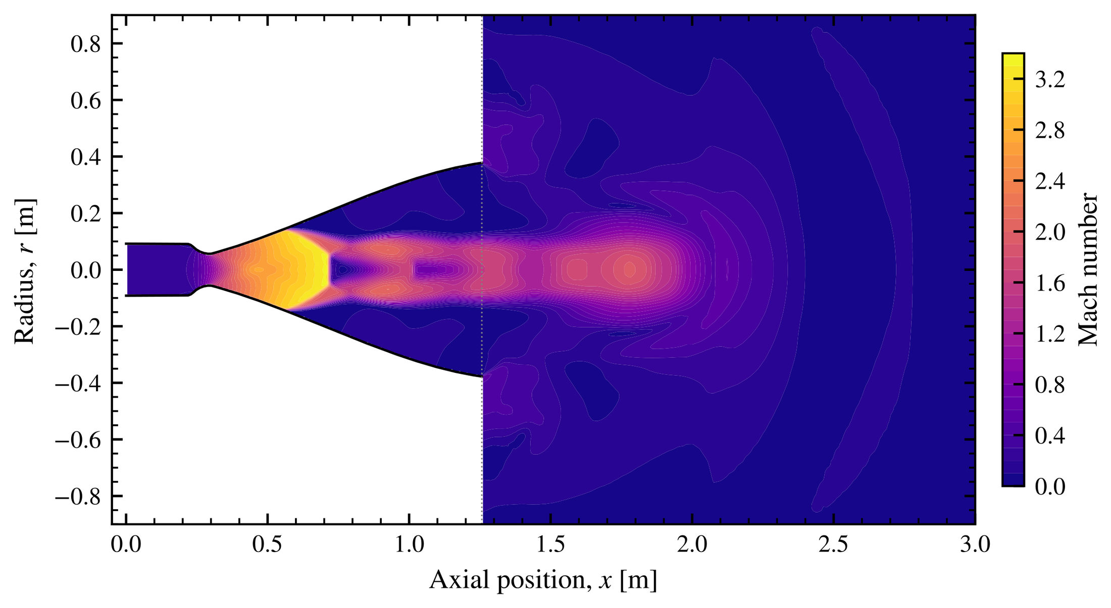
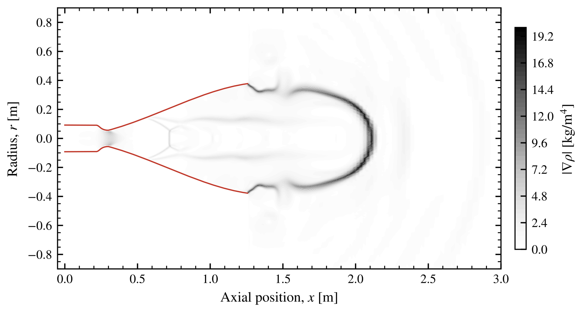
Fig. 10 — Case 05 at sea-level start-up: separated flow and a Mach disc inside the bell, and the jet pushing out into the room.

Fig. 11 — The same moment in numerical schlieren. The starting-jet front is a curved, shock-like front well ahead of the nozzle lip.

I tracked where Z = 0.5 crosses the axis. After 5 to 6.5 ms, the front was only 1.05 to 1.80 exit diameters past the lip. It advanced at about 377 m/s, against roughly 2,900 m/s inside the duct. This is the early starting jet, before a plume develops.

A physical diagnostic caught what the residuals did not. Each leg simulated only half a millisecond, but a pressure wave needs about 20 ms to cross from the far-field boundary. As a result, the lower ambient pressures never reached the jet. The same case also produced a 778 GB log that filled the disk and crashed the virtual machine. The cause was an over-hot initial condition that exceeded the 3,600 K limit of the thermodynamic fit on every step. Both were worth learning the hard way.

References

[1]J. C. Hooper III, Performance Analysis of the Ascent Propulsion System of the Apollo Spacecraft, NASA TN D-7400, 1973; C. E. Humphries and R. E. Taylor, Apollo Experience Report: Ascent Propulsion System, NASA TN D-7082, 1973. (Engine background and operating point.)
[2]G. P. Sutton and O. Biblarz, Rocket Propulsion Elements, 9th ed., Wiley, 2017.
[3]J. D. Anderson, Modern Compressible Flow with Historical Perspective, 3rd ed., McGraw-Hill, 2003.
[4]C. J. Greenshields, H. G. Weller, L. Gasparini and J. M. Reese, “Implementation of semi-discrete, non-staggered central schemes in a colocated, polyhedral, finite volume framework, for high-speed viscous flows,” Int. J. Numer. Methods Fluids 63, 1–21, 2010.
[5]A. Kurganov and E. Tadmor, “New high-resolution central schemes for nonlinear conservation laws and convection–diffusion equations,” J. Comput. Phys. 160, 241–282, 2000.
[6]F. R. Menter, “Two-equation eddy-viscosity turbulence models for engineering applications,” AIAA J. 32, 1598–1605, 1994.
[7]T. J. Poinsot and S. K. Lele, “Boundary conditions for direct simulations of compressible viscous flows,” J. Comput. Phys. 101, 104–129, 1992.
[8]J. S. Turner, “The ‘starting plume’ in neutral surroundings,” J. Fluid Mech. 13, 356–368, 1962.
[9]D. G. Goodwin, H. K. Moffat, I. Schoegl, R. L. Speth and B. W. Weber, Cantera, v3.0, 2023.