What the Grid Can’t See: Recovering Unresolved Turbulence
Independent computational studyEvery practical turbulence simulation discards the small scales and then has to guess what they were doing. This personal project asks a sharper question. If you watch the large scales for a while, how much can you actually say about the small ones, and how confident can you be? The study has three parts: my own RANS and LES runs, an in-house turbulence solver, and information-based measures of what coarse data determines. I scored my runs against published DNS, experiment and LES data.
WhatThe closure problem, in one picture
Split any turbulent velocity into a mean and a fluctuation, then average the Navier–Stokes equations. A new term appears: the Reynolds stress. It is the average effect of all the small, fast motions on the large, slow ones [1]:
The Reynolds-averaged momentum equation. Everything is known except the last term, \(\langle u_i'u_j'\rangle\), which depends on the very motions that the average removed. That missing piece is the closure problem.
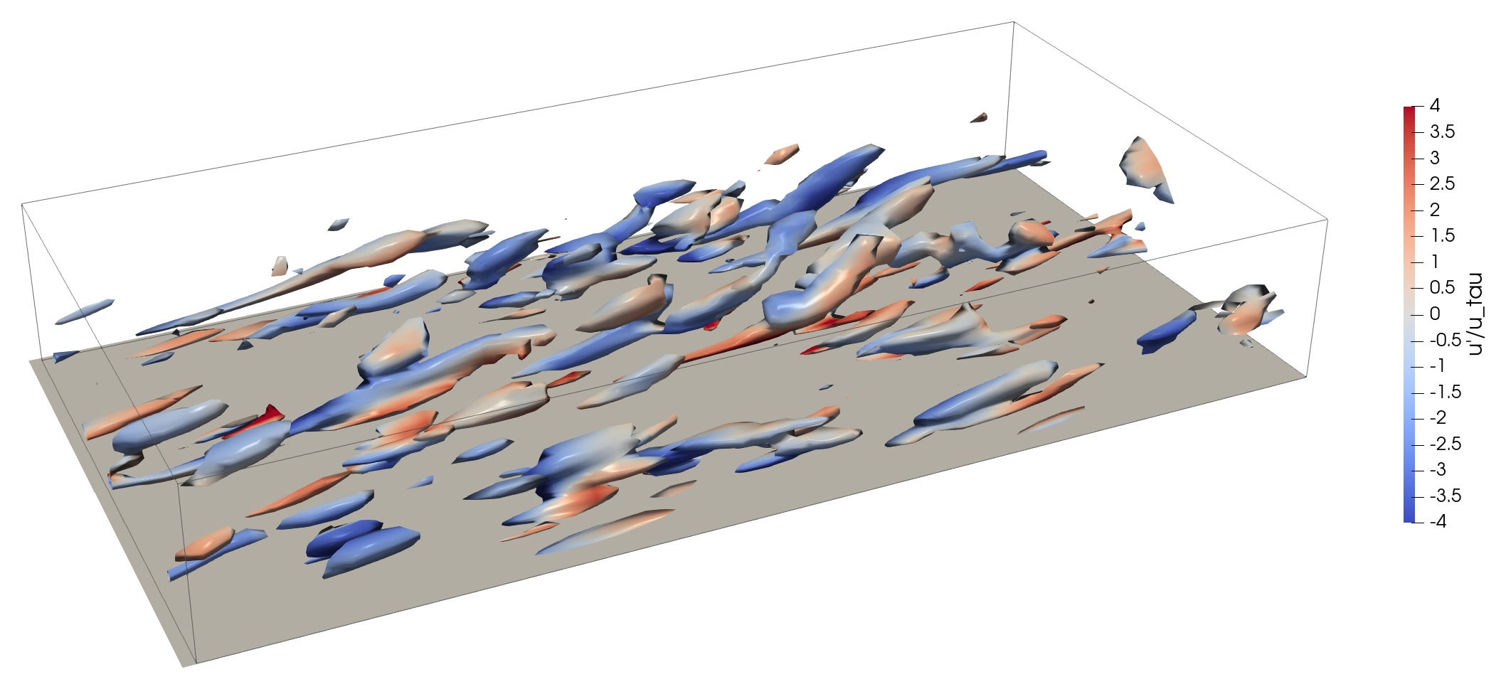
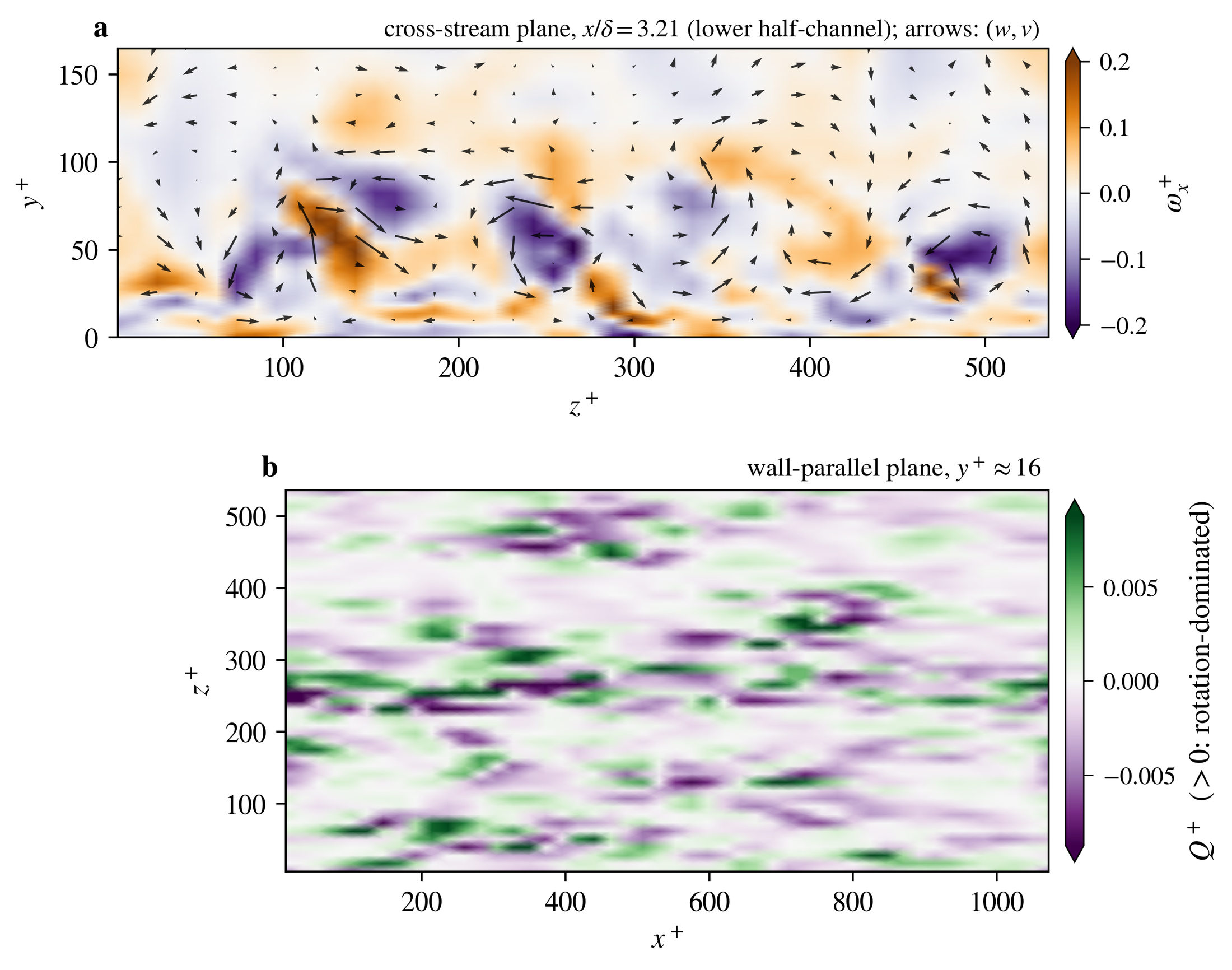
A RANS model replaces that term with a formula. An LES resolves the large eddies and models only what is smaller than the grid. Either way, part of the flow is never computed, and the model has to stand in for it. The physical picture of what is lost is striking:
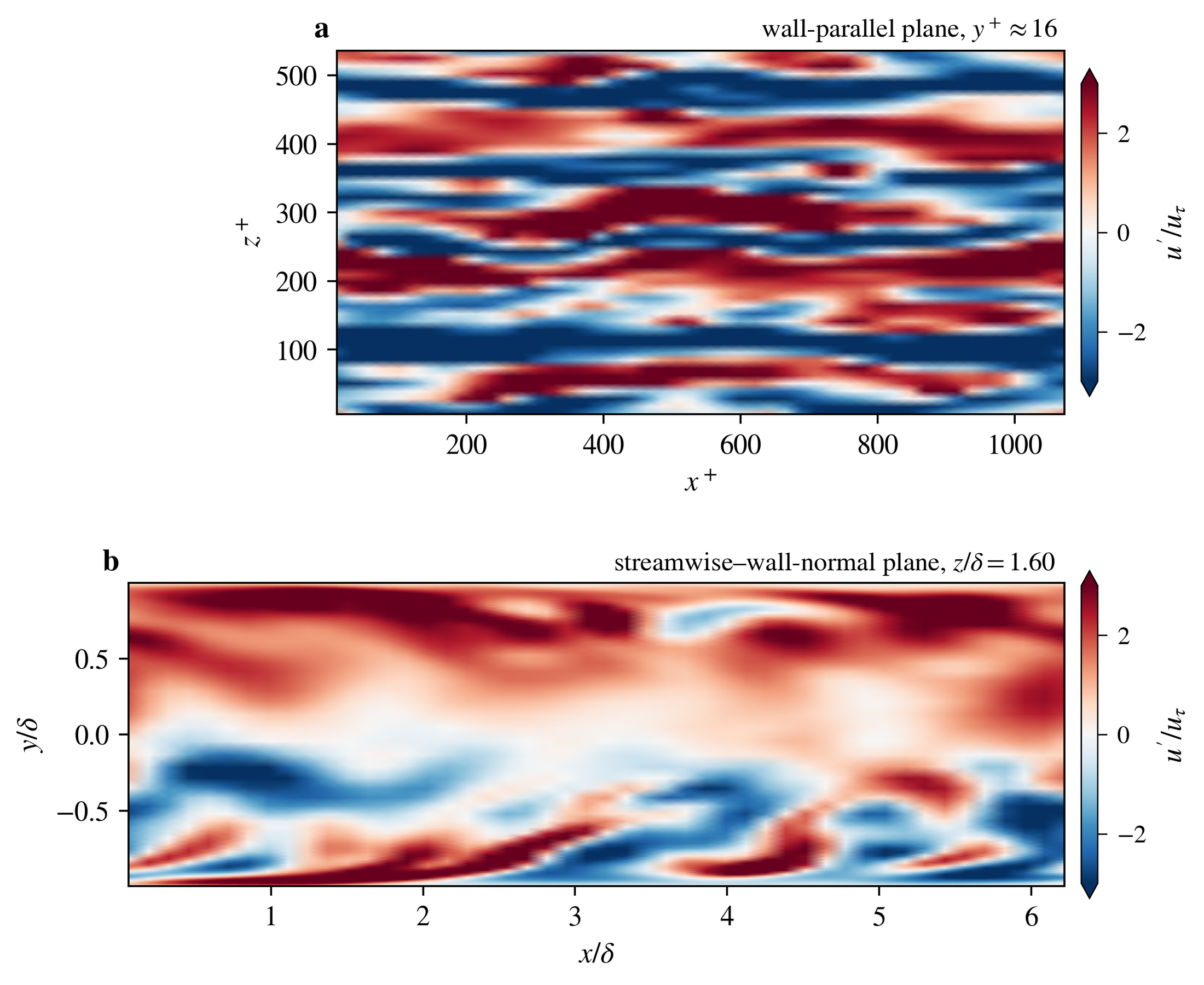
Those streaks, and the vortices that lift them, are the machinery of wall turbulence. A RANS model sees none of them, only their average effect. This project asks how much of that machinery can be recovered from coarse information, honestly and with a measured uncertainty. It asks this especially when the coarse information arrives as a history.
HowStep 1 · Know what the models get right and wrong
Before I tried to recover anything, I needed to know how good the usual models are. I ran unmodified OpenFOAM cases and scored them against public reference data. The data are channel-flow DNS, the NASA wall-mounted hump experiment and a published LES of the hump [2, 3, 4]. For the LES runs, I wrote down the accuracy criteria before I ran them, so I could not tune the result after the fact. The LES uses the WALE subgrid model, which vanishes near walls, as it should [6]:
The WALE eddy viscosity is built from the traceless symmetric part of the squared velocity gradient, \(S^d_{ij}\), so it vanishes in pure shear at a wall. The second expression is the normalized error used to score each profile against DNS.
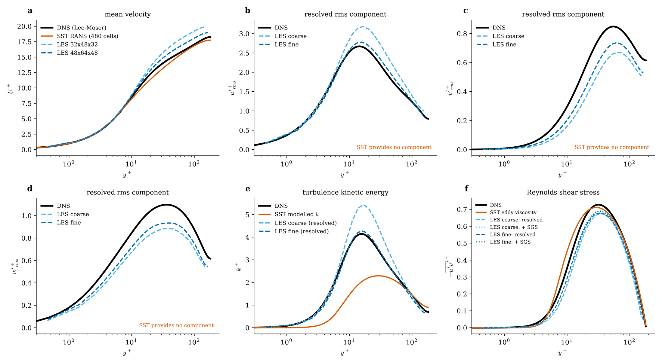
The channel results are a useful reality check. With 147,000 cells, the LES gets the peak turbulent kinetic energy within 4% of DNS (4.3 vs 4.15 in wall units) and the streamwise fluctuations within 4%. But the wall-normal and spanwise fluctuations are 13% and 15% low, and the LES met two of the three criteria that I had set. SST RANS gets the mean velocity within 2–3.5% of DNS at every Reynolds number from Reτ = 182 to 5186. Yet its turbulent kinetic energy peaks at only 54–58% of the true value. Good means, wrong turbulence is the pattern that a closure model hides.
HowStep 2 · A separated flow, where models disagree
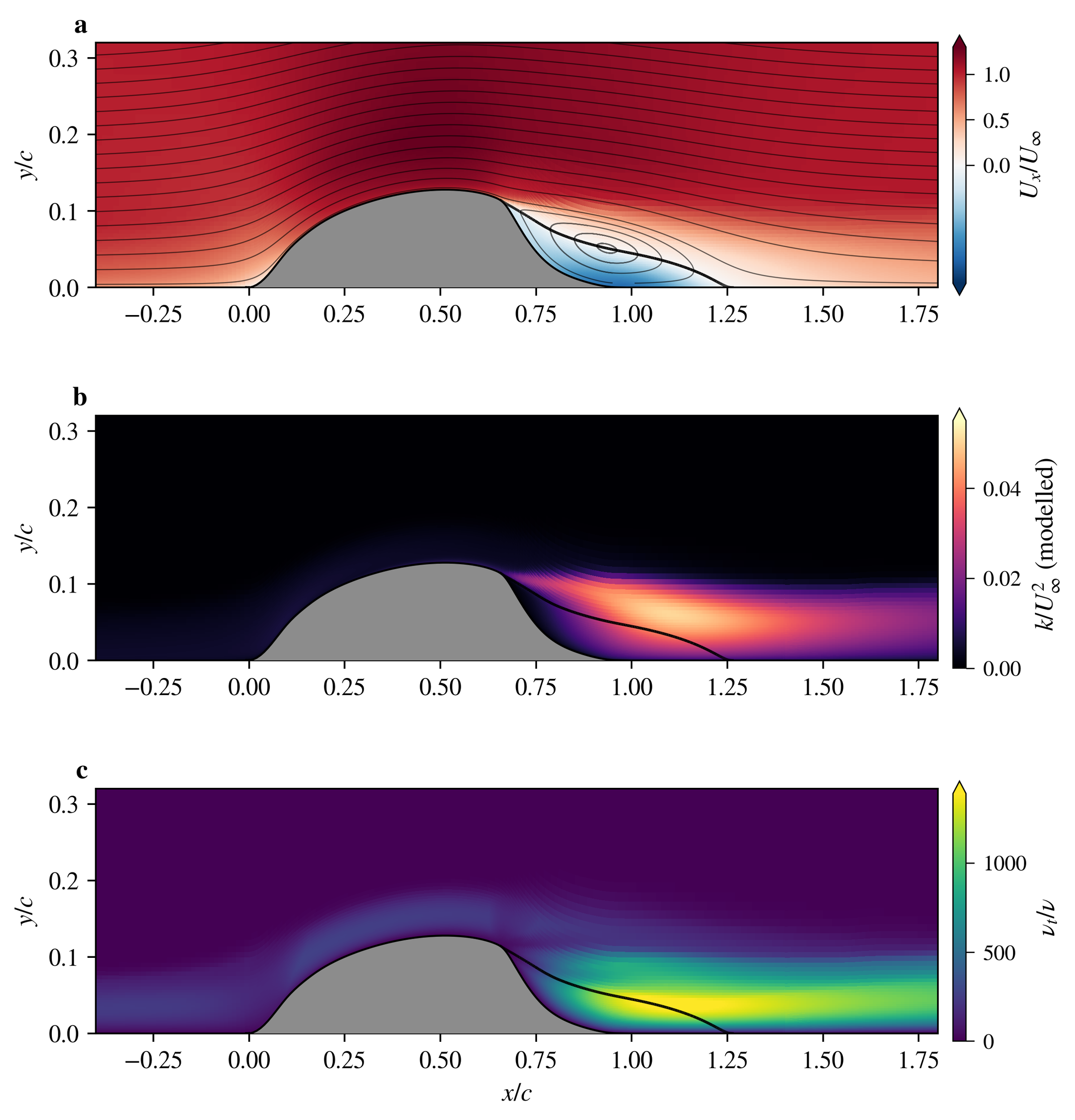
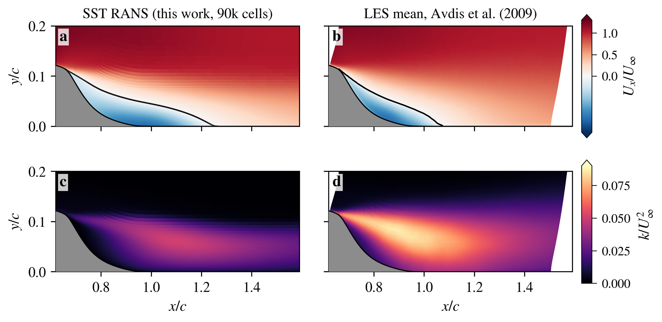
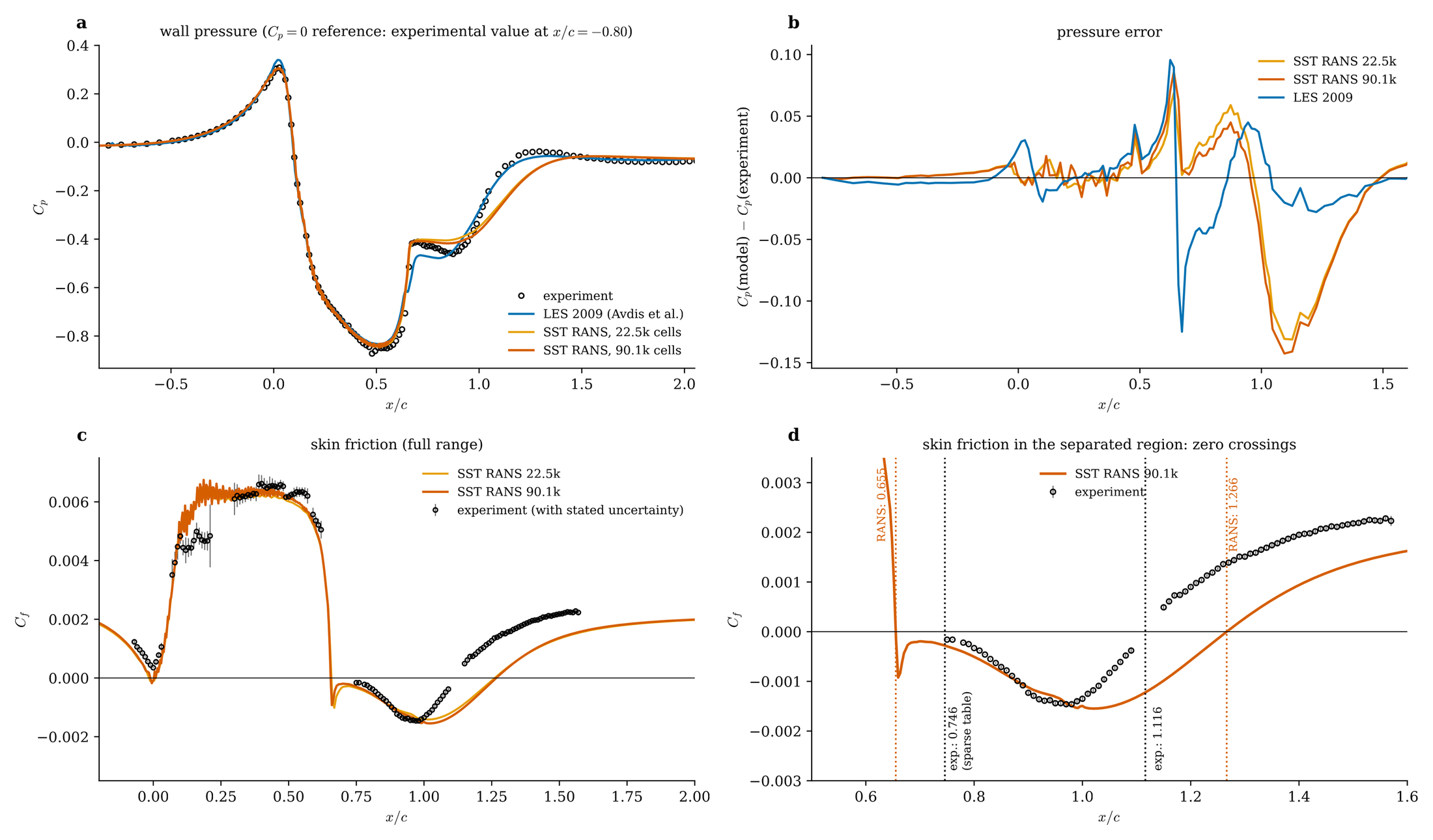
Separation is where turbulence models are tested hardest. Over the NASA hump, SST gets the suction peak almost right (Cp −0.847 against −0.872 measured). But its bubble reattaches 13% too late (x/c 1.266 vs 1.116), because its shear-layer turbulence is too weak. Its peak k is about 0.050 U∞², against 0.087 U∞² in the published LES [4, 5]. The published LES, in turn, over-predicts the measured stresses by 40–50% in the same region. The experiment sits between the two models, so neither model is a trustworthy stand-in for the true unresolved state.
A flat-plate case verifies the pipeline itself. Skin friction is within 4.1% of the White correlation after Richardson extrapolation, with a grid-convergence index of 2.4% [11].
HowStep 3 · My own turbulence, to test ideas on
To test reconstruction ideas, I need turbulence where I know the full truth. I built a GPU pseudo-spectral Navier–Stokes solver for forced, triply periodic turbulence. It is verified on the Taylor–Green vortex, it is stationary to 1%, and it closes its energy budget to 0.7%.
The hardware is the same gaming laptop that I describe on the Sandia Flame D page. It caps the forced-turbulence testbed at 32³ to 64³ grids and modest Reynolds numbers. That is small for turbulence work, so every run has to earn its place.
Kolmogorov’s inertial-range spectrum, the Kolmogorov length scale, and the velocity-derivative skewness [8]. A negative skewness is the statistical signature of energy that cascades to small scales.
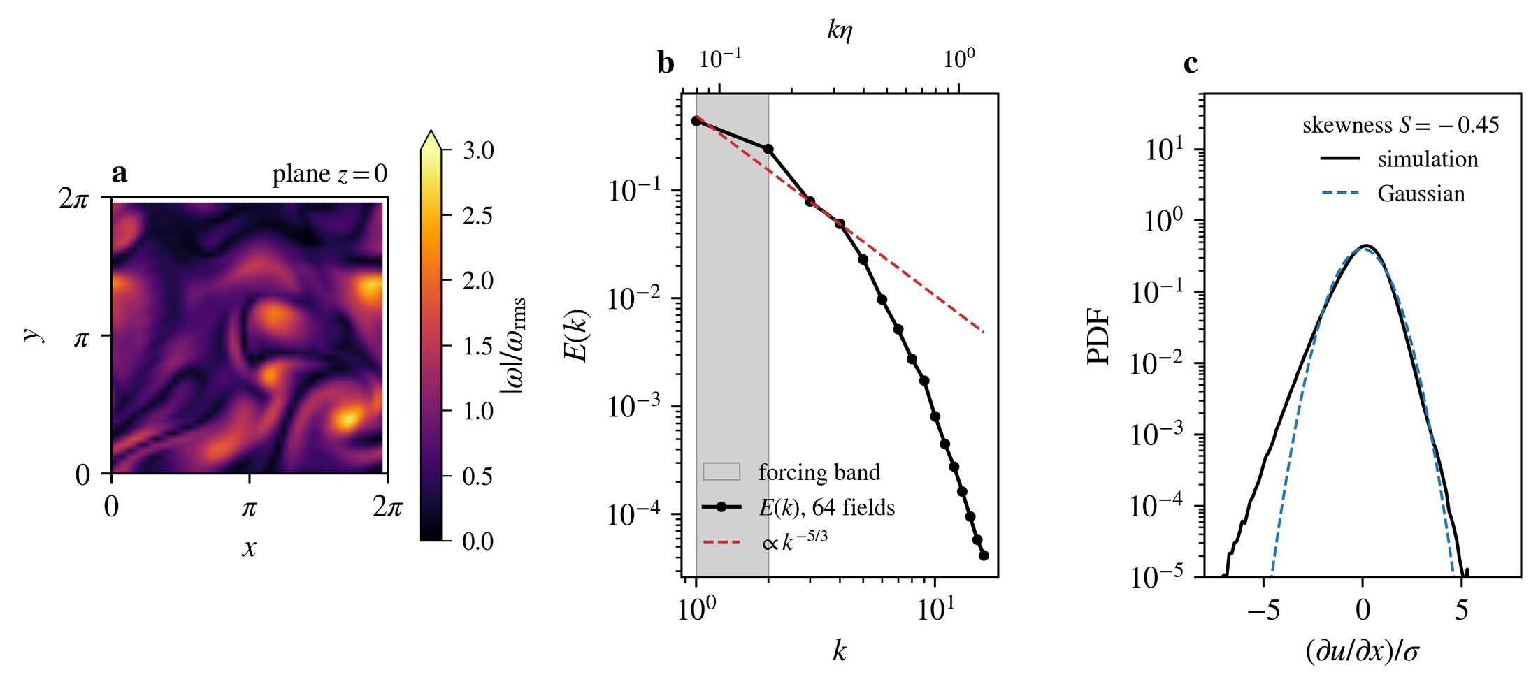
At this modest Reynolds number, the spectrum follows the −5/3 slope only over a short band, as expected. But the small-scale statistics already look like real turbulence. The velocity-derivative skewness is −0.45 ± 0.15, close to the −0.5 commonly reported, and the gradient PDF has the heavy tails that a Gaussian lacks.
ResultsWhy coarse data cannot pin down turbulence
A simple experiment shows the core difficulty. I start from eight random, band-limited 3-D velocity fields on an 18³ grid. For each one, I make 24 copies that keep every Fourier amplitude and change only the phases. At that first instant, all copies of a field have the same energy, spectrum and dissipation. I then let every copy evolve freely, without forcing, for 0.6 s.
After that evolution, I split the variance of each statistic into two parts. One part is between the original fields, and the other is between phase copies of one field. The phase share is the part that the starting amplitudes do not determine. Energy-type statistics barely depend on the phases. The statistics that describe how turbulence works depend on them strongly:
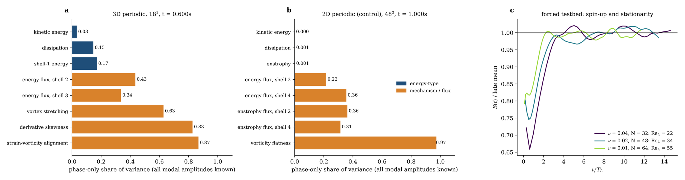
This is an exploratory check. The starting fields are random Gaussian fields, and the flow decays. In 2-D, the energy-type share is below 0.1%, which is consistent with a three-dimensional effect. But the 2-D run uses a different viscosity, grid and elapsed time, so that contrast is only suggestive.
A good coarse model aims roughly to match a spectrum. In this test, a matched starting spectrum left the vortex stretching that drives the cascade largely undetermined. That is why the answer has to be a distribution of possible small-scale states. It is also why I score it with information measures [9]:
The Kullback–Leibler divergence between a true and a predicted Reynolds-stress covariance (treated as Gaussians). Roughly, it is the number of nats of information that the prediction is missing. Zero means a perfect match.
To calibrate that scale, I measured classical algebraic stress models with standard constants. In channel flow, they recover 44–70% of the information gap between an isotropic eddy-viscosity guess and the DNS stresses. The share rises with Reynolds number. That is a measurement of textbook models.
ResultsEarly evidence: history helps, in an idealized test
Each reconstruction is an ensemble. I score it with the continuous ranked probability score, which rewards a result that is both accurate and honestly uncertain. The score is relative to a simple guess from long-run statistics [10]:
The first term penalizes ensemble members far from the truth \(y\). The second term rewards appropriate spread. A skill ratio \(S\) below 1 means that the observations carry real information.
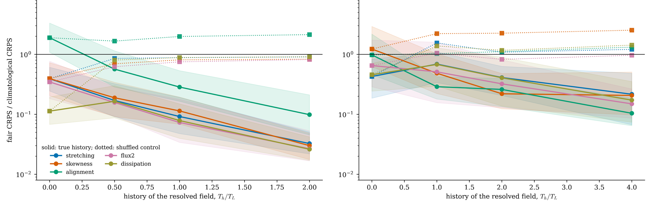
In the in-house turbulence, 10% of the energy is hidden. Consider the score for vortex stretching a quarter of an eddy turnover ahead. It falls from 0.39 with no history to 0.033 with two turnover times of history. That is a roughly tenfold improvement. With the history of a different flow instead, the score stays at 0.86–0.91. The gain comes from the information in the history (Result view at the top). With 20% hidden, four turnover times of history are necessary to reach 0.10–0.22.
These numbers come from a deliberately idealized setting. The truth is my own simulation and the observations are exact. The reconstruction also had the true small-scale energy spectrum, so only the phases were unknown. The results support the idea only inside this idealized setting. They are not a practical result. Not everything worked: in the first small nonlinear test, history made the score slightly worse (0.0713 → 0.0784 m/s), and that result stays on the record.
References
- [1]S. B. Pope, Turbulent Flows, Cambridge University Press, 2000.
- [2]M. Lee and R. D. Moser, “Direct numerical simulation of turbulent channel flow up to Reτ ≈ 5200,” J. Fluid Mech. 774, 395–415, 2015.
- [3]D. Greenblatt, K. B. Paschal, C.-S. Yao, J. Harris, N. W. Schaeffler and A. E. Washburn, “Experimental investigation of separation control, Part 1: baseline and steady suction,” AIAA J. 44, 2820–2830, 2006.
- [4]A. Avdis, S. Lardeau and M. Leschziner, “Large eddy simulation of separated flow over a two-dimensional hump with and without control by means of a synthetic slot-jet,” Flow Turbul. Combust. 83, 343–370, 2009.
- [5]F. R. Menter, “Two-equation eddy-viscosity turbulence models for engineering applications,” AIAA J. 32, 1598–1605, 1994.
- [6]F. Nicoud and F. Ducros, “Subgrid-scale stress modelling based on the square of the velocity gradient tensor,” Flow Turbul. Combust. 62, 183–200, 1999.
- [7]J. C. R. Hunt, A. A. Wray and P. Moin, “Eddies, streams, and convergence zones in turbulent flows,” Proc. Summer Program, Center for Turbulence Research, Stanford, 193–208, 1988.
- [8]A. N. Kolmogorov, “The local structure of turbulence in incompressible viscous fluid for very large Reynolds numbers,” Dokl. Akad. Nauk SSSR 30, 301–305, 1941.
- [9]T. M. Cover and J. A. Thomas, Elements of Information Theory, 2nd ed., Wiley, 2006.
- [10]T. Gneiting and A. E. Raftery, “Strictly proper scoring rules, prediction, and estimation,” J. Am. Stat. Assoc. 102, 359–378, 2007.
- [11]F. M. White, Viscous Fluid Flow, 3rd ed., McGraw-Hill, 2006.