Sandia Flame D: What a Reactor Network Discards

Home / Projects / Independent computational studies

Mean temperature of my RANS/EDC simulation of Sandia Flame D, on its own mesh and mirrored about the axis

Two ways to cut the same flame into eight reactors: by composition (k-means, top) and by where the mass flows (flux-coherent, bottom)

The final network: eight reactors at their cluster centroids, the measured mass fluxes between them, and CFD vs network temperature at each node

Sandia Flame D: What a Reactor Network Discards

Independent computational study

A personal learning project on a simple question: how much of a turbulent flame survives when you reduce it to a few chemical reactors? I set it up as four steps, each with a check before the next. I built the CFD, built reactor networks from it, measured what the reduction throws away, and tested ways to put it back. The networks are scored against my own parent CFD. Only the CFD and the tabulated chemistry are scored against the experiment.

What worked

A mass-exact network with no fitted parameters (R²(T) = 0.71 against the parent CFD). An exact split of what averaging discards, and a parameter-free closure that recovers much of it (R²(T) 0.82, CO 0.73, also against the parent CFD). Tabulated chemistry, applied a priori to the frozen CFD fields, that raises temperature agreement with the experiment from R² 0.40 to 0.61.

What did not

Mean-state networks at realistic mixing (they extinguish). CO in every surrogate. A learned correction that did not transfer to an unseen region of the flame. The parent CFD itself over-predicts near-field temperature, and every surrogate inherits that bias.

Methods & tools

OpenFOAM (reactingFoam, k–ε, EDC, TDAC/ISAT) · ParaView · Cantera with detailed CRECK chemistry · PCA, k-means and spectral clustering · presumed β-PDF tabulation · conditional (CMC-style) closure · bootstrap and hold-out tests

Project breakdown

WhatThe question and the plan

Reactor networks carry detailed chemistry at almost no cost. Our group’s RQL combustor model uses one [8]. That speed matters to me for a practical reason: I run everything on an ASUS TUF F15 laptop with an RTX 3050 Ti. A fine 3-D LES of a flame is out of reach, so reduced-order models are how I get detailed chemistry at all. Honestly, it sucks, but it also makes for a fun problem.

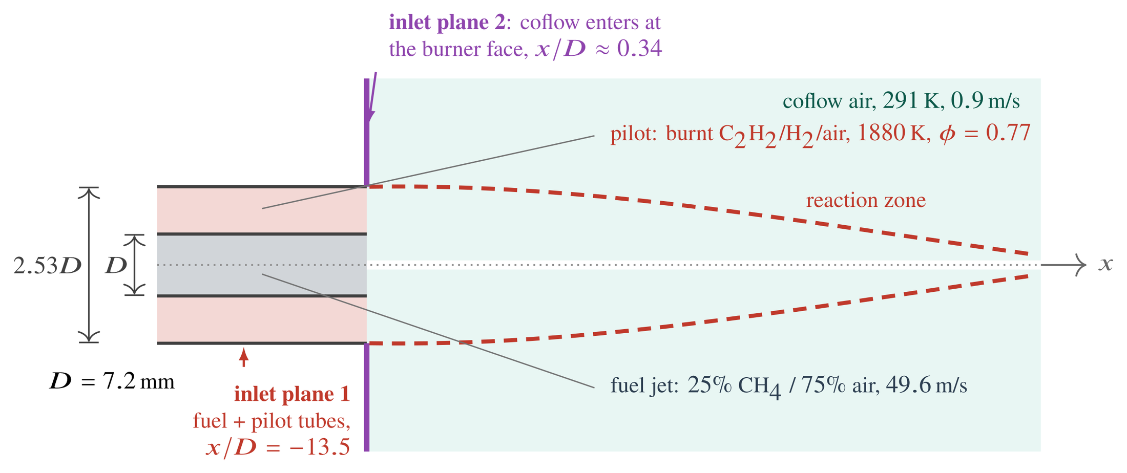
Sandia Flame D is the right test case. It is a piloted methane/air jet flame with temperature, species and velocity measured across the whole flame [1]. Other groups have also built reactor networks for it [6]. I planned four steps:

Step 1. Build a parent CFD solution and measure how good it is against the experiment.
Step 2. Build a reactor network from that solution.
Step 3. Measure what the reduction throws away.
Step 4. Test ways to recover it, including tabulated chemistry.

Every network result had to pass three checks. It must hold at the physical flow rate, use measured boundary conditions, and hold on data it was not fitted to. These checks turned out to be the most useful part of the project.

HowStep 1 · The parent simulation

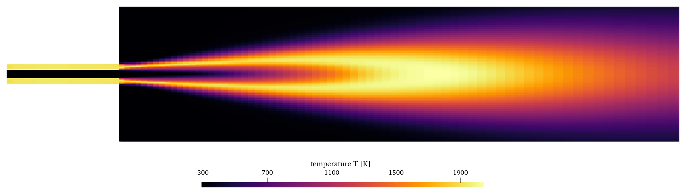
Fig. 1 — The burner: a 25% CH₄ / 75% air jet at 49.6 m/s (D = 7.2 mm, Re ≈ 22,400). The burner also has a burnt pilot at 1880 K and a slow air coflow.

I set up a steady RANS simulation in OpenFOAM on a 5° axisymmetric wedge of 5,170 cells. It uses standard k–ε turbulence and the Eddy Dissipation Concept, with a 36-species GRI-3.0 subset [2, 3, 4]. The mesh is coarse on purpose, because the laptop has to solve it with detailed chemistry.

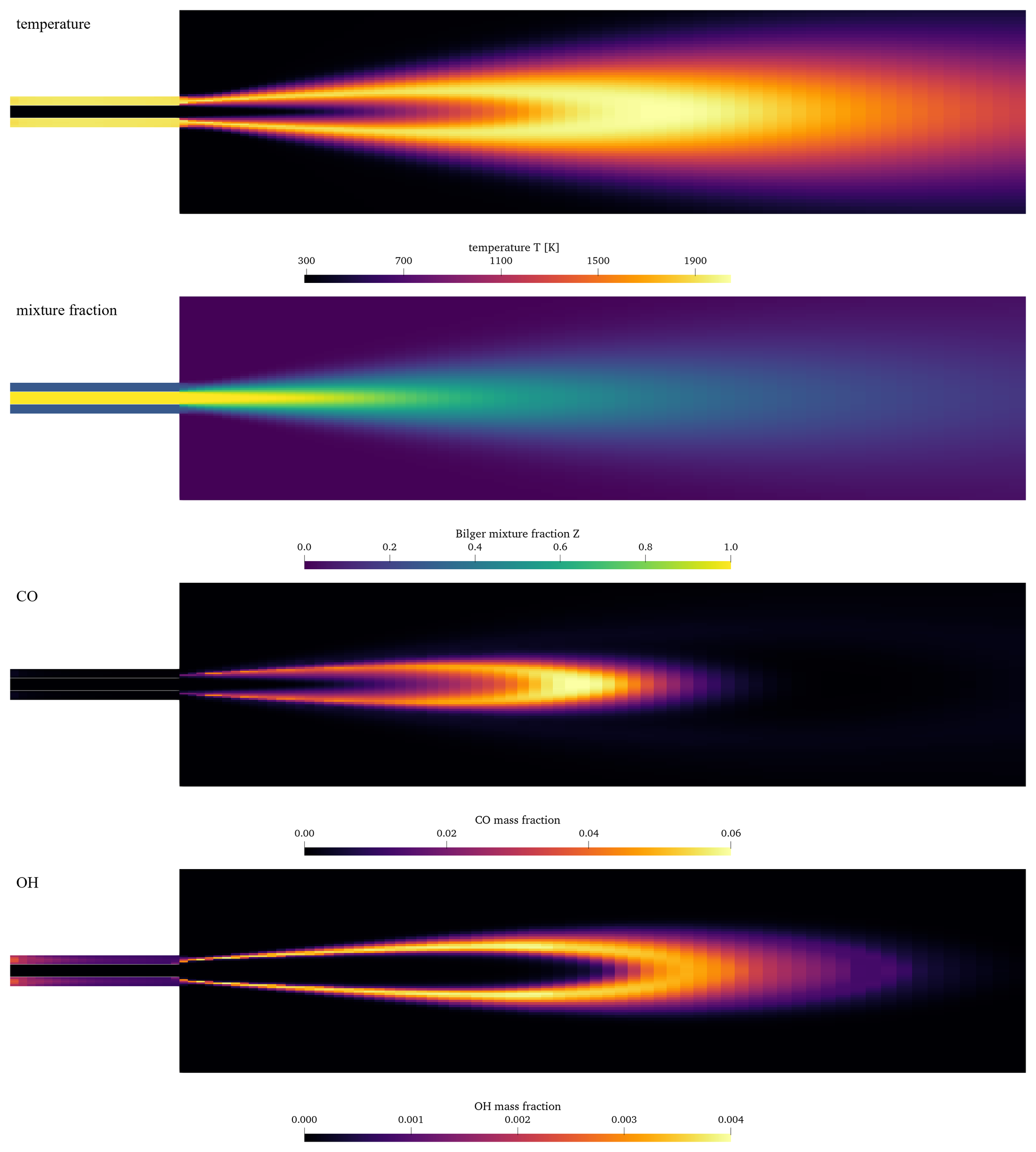
Fig. 2 — Anatomy of the simulated flame: temperature, mixture fraction, CO and OH, each with its own color scale (mirrored about the axis, x from −0.10 to 0.50 m).

The four fields show the structure a network has to represent. Mixture fraction marks where fuel and air meet. The hot sheath sits on the stoichiometric surface. CO forms in a tongue on the rich side, and OH lives in a thin sheet where burnout happens.

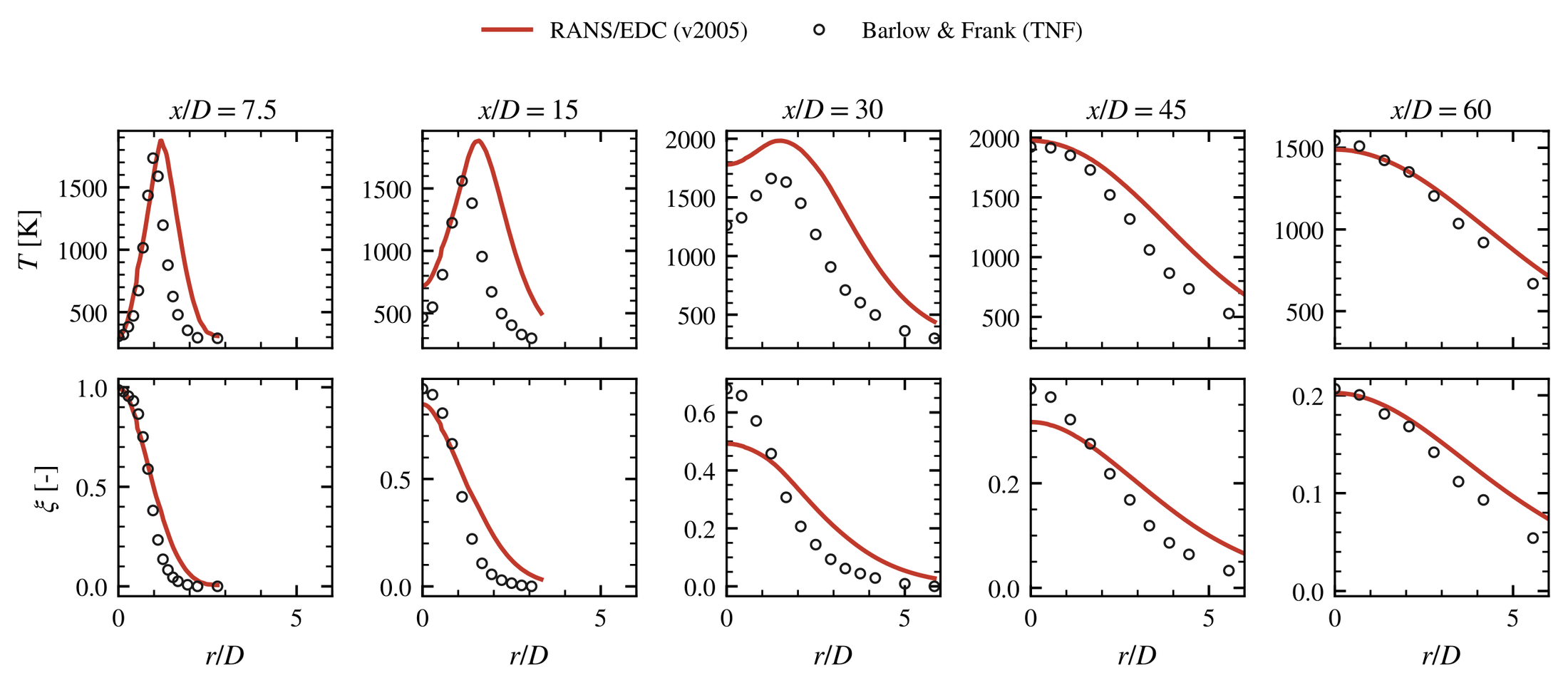
Against the TNF measurements, velocity (centerline R² 0.93) and mixture fraction (R² 0.91) agree well. Temperature is too high by 283 K on average (R² 0.40) and worst at x/D = 15. I attribute this to the known tendency of k–ε to over-mix the near field. CO reaches only R² 0.20. This is therefore a converged baseline with a known near-field bias. Every surrogate inherits that bias, so I scored the networks against the CFD and kept the experiment as a separate check.

Radial temperature and mixture fraction at five stations: the RANS/EDC solution (line) against the Barlow & Frank measurements [[1]] (circles). — Fig. 3 — Radial temperature and mixture fraction at five stations: the RANS/EDC solution (line) against the Barlow & Frank measurements [1] (circles).

HowStep 2 · From a CFD field to a reactor network

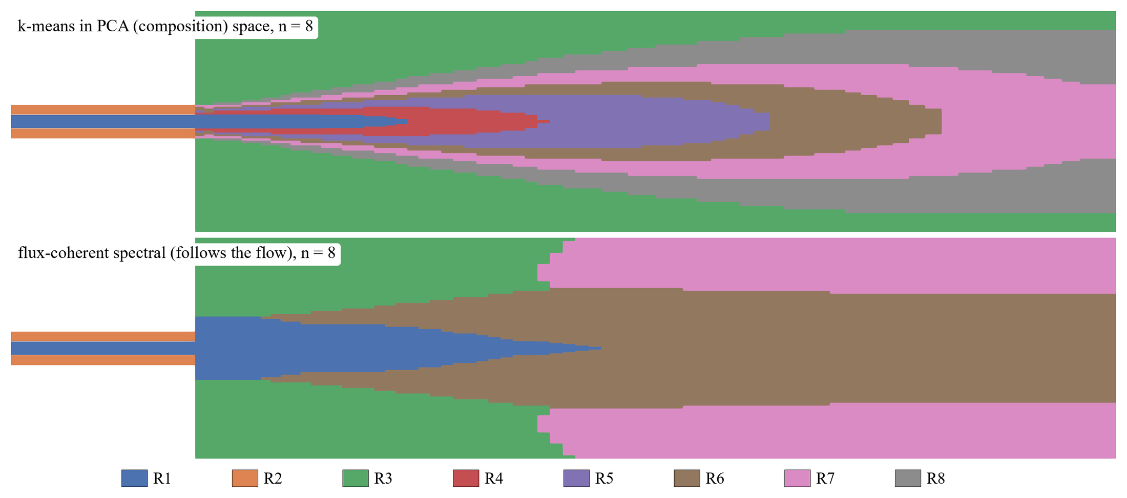
I cluster the cells into eight reactors. The reactor volumes come from the cell volumes, and the connections come from the CFD face fluxes. A turbulent Damköhler number sets each reactor as stirred or plug-flow [8]. The Method view at the top shows the two clustering choices I compared: by composition and by mass flow.

Any network has two built-in losses. A reactor computes chemistry only at its own mean state, and one interface carries one state for every cell face it replaces:

\[\omega\!\left(\langle\mathbf Y\rangle_i\right)\neq\left\langle\omega(\mathbf Y)\right\rangle_i,\qquad \Big(\textstyle\sum_{f\in\Gamma_{ij}}K_f\Big)\big(\bar Z_i-\bar Z_j\big)\;\neq\;\sum_{f\in\Gamma_{ij}}K_f\big(Z_{P,f}-Z_{N,f}\big)\]

Chemistry at the mean is not the mean of the chemistry, because reaction rates are strongly nonlinear [9]. Exchange computed from two cluster means is not the sum of the face exchanges it replaces (\(K_f\) is the turbulent conductance of each face).

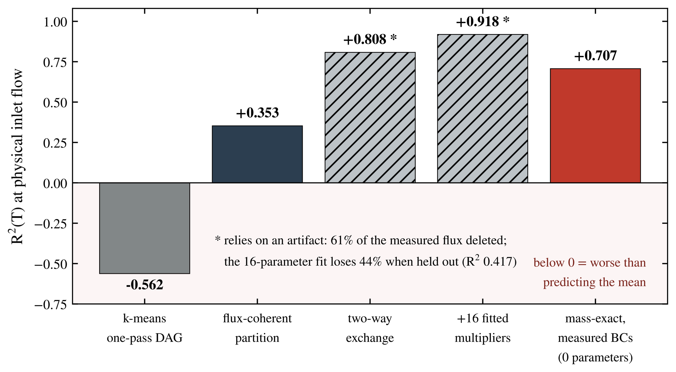
Fig. 4 — Network temperature R² against the parent CFD at the physical flow rate, at each stage. The two starred values failed the checks and were withdrawn. The final network has no fitted parameters.

The three checks did their job. They caught three results that looked good for the wrong reasons:

A composition-based network scored R² ≈ 0.8, but only at 1/200 of the real inlet flow. At the physical flow rate it scored −0.56.
A mass-balance repair raised R² to 0.81, but it deleted 61% of the measured flux between clusters.
Sixteen fitted multipliers gave 0.92 in the fit, but only 0.42 on held-out data.

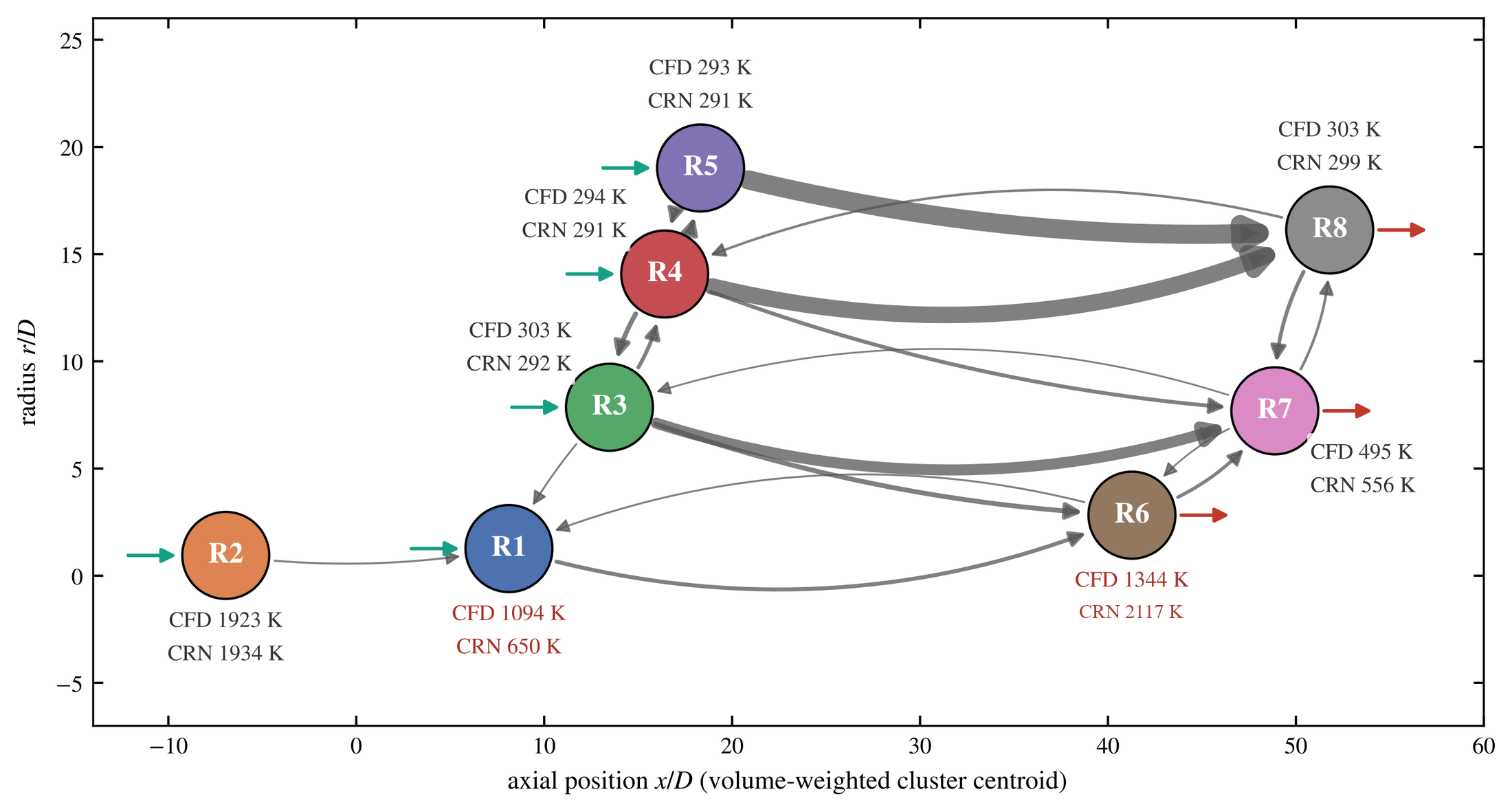
Clustering by mass flow instead of composition removed the first problem, because the network then carried the real flow through the flame. The result is the network in the Result view: measured boundary fluxes, mass closed to 4×10⁻¹⁹ kg/s, no fitted parameters, and R²(T) = 0.71. That score is against the parent CFD. Most of the remaining error sits in two reactors.

These network scores are R² over eight cluster means at one operating condition, so one cluster can dominate them. They measure agreement with the parent CFD. Agreement with the experiment is a separate question.

ResultsStep 3 · What the reduction throws away

Exchange between two clusters splits exactly into a part the network keeps (the difference of the cluster means) and a part it discards (how far each cluster’s edge state is from its own mean):

\[\dot J_{ij}=K_{ij}\Big[\underbrace{\big(\bar Z_i-\bar Z_j\big)}_{\text{kept}}+\underbrace{\big(\delta Z_{i,ij}-\delta Z_{j,ij}\big)}_{\text{discarded}}\Big],\qquad \delta Z_{i,ij}=\frac{\sum_f K_fZ_{i,f}}{K_{ij}}-\bar Z_i\]

Exact to \(6.5\times10^{-19}\) kg/s. A cluster shows a different state to each neighbor, so no single mean can represent all of them.

The discarded part is large: the lumped model over-states the gradient at the interfaces by about 14×. A first-order reconstruction inside each cluster (P1) puts much of it back with no fitted parameter. I also gave the network the true edge states (an “oracle”) to see the ceiling.

Fig. 5 — Mixture fraction from the CFD, cell by cell (top). The next panels show the eight-reactor solution with the calibrated lumped closure, with P1 (no fitted parameter) and with the oracle edge states (diagnostic ceiling).

≈ 14×interface gradient over-stated by the lumped model

0.64 → 0.82R²(T) against the parent CFD, calibrated lumped model → P1

0.93R²(T) ceiling with the true edge states (diagnostic only)

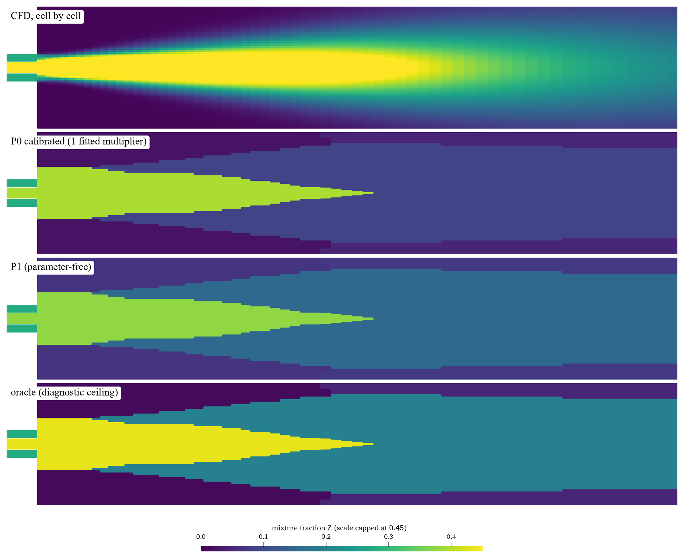
P1 has limits. It is not bounded (one cluster solves at a slightly negative mixture fraction), and it is sensitive to its weighting. Mean-state reactors also have a hard limit: with realistic turbulent mixing between them, every reactor except the pilot extinguishes. R²(T) against the CFD falls from 0.71 to 0.39. Hot and cold starts give the same answer, so this is a real fixed point of the model. Within the network family I tested, mean-state reactors cannot represent this flame at realistic mixing rates.

ResultsStep 4 · Chemistry from tables

The other way to recover what averaging loses is to never compute chemistry at a mean. I tabulated well-stirred-reactor solutions in mixture fraction and residence time. Then I averaged them over a presumed β-PDF and blended fresh and burnt states with a progress variable [5]:

\[\tilde f=\int_0^1 f(\zeta)\,P_\beta(\zeta;\bar Z,\widetilde{Z''^2})\,d\zeta,\qquad f=(1-c)\,f_{\mathrm{fresh}}+c\,f_{\mathrm{burnt}}\]

β-PDF average over the mixture-fraction fluctuations, and the blend between unburnt and burnt states with progress variable \(c\).

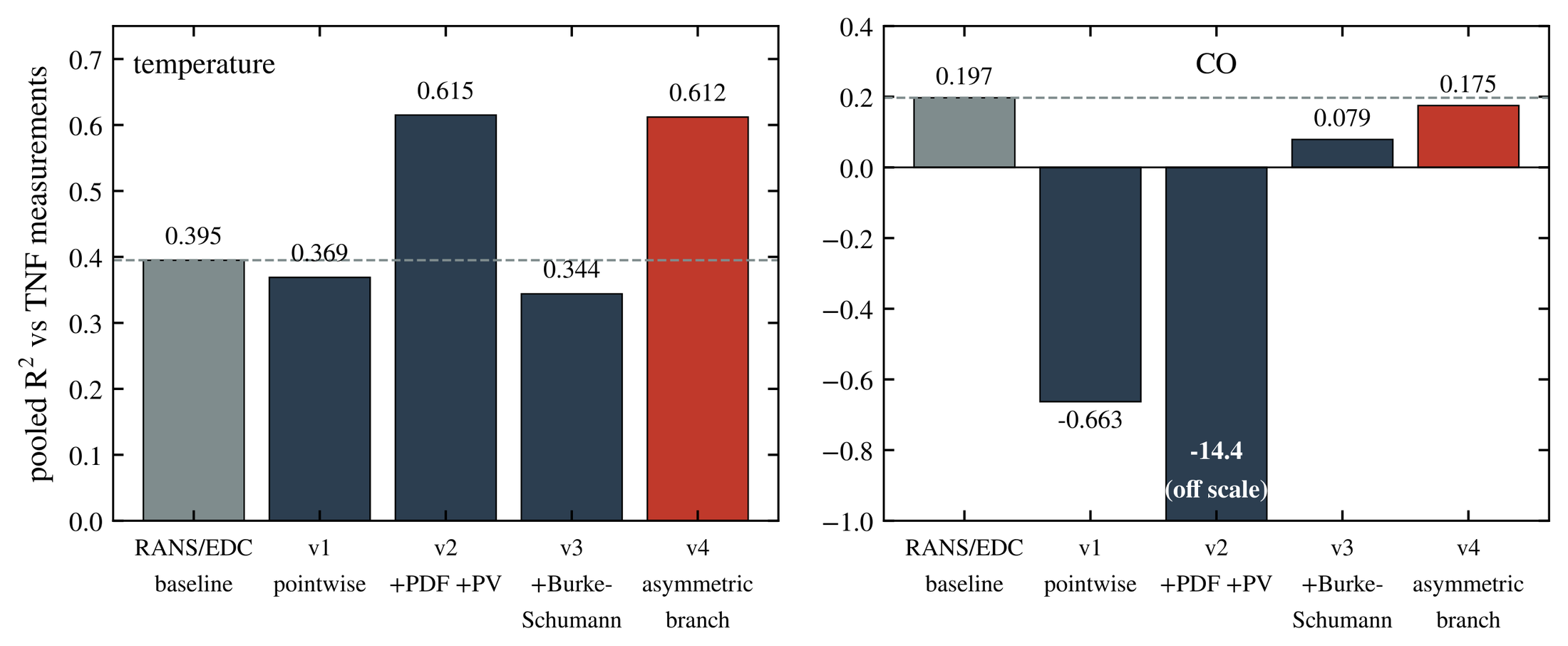
Fig. 6 — Pooled R² against the TNF measurements for temperature and CO: the RANS/EDC baseline, then each table version. Each version targets the failure found in the one before.

Four table versions raised temperature agreement with the experiment from R² 0.40 to 0.61 (0.57 when each measurement station is held out). CO did not follow. It reached 0.18, just below the EDC baseline of 0.20.

These are a-priori tests. I applied the table to the frozen CFD fields, and its progress variable comes from the CFD species. The table is therefore a conditioned reconstruction. It also uses one calibrated constant, and its grid in mixture fraction and residence time is not converged.

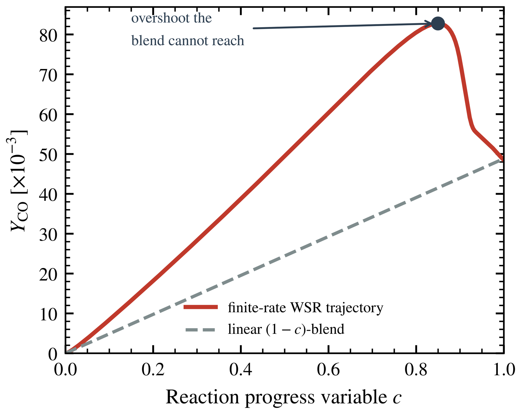
Fig. 7 — A likely reason CO fails: in a stoichiometric finite-rate reactor, CO overshoots to about 1.7× its burnt value near c ≈ 0.85. No linear progress-variable blend can reach that peak.

My explanation for the CO failure comes from reactor calculations. I have not proven it. CO rises past its burnt value before it burns out, almost all through CO + OH → CO₂ + H. At the CO peak, OH sits at 2.4× its equilibrium value. A surrogate that assumes an equilibrium burnt state therefore uses the wrong radicals. Coarse networks also average away this produce-then-consume structure. Published work on this flame needs hundreds to thousands of reactors to resolve CO [7].

Tracking down that explanation was the best part of the project. I think it is kind of sick that one reaction path accounts for so much of the failure.

A learned model can predict the discarded edge states inside this flame (skill 0.86), but it fails on an axial region it has not seen (−0.12). For that reason, I did not use a learned closure. All results here are for one flame at one operating condition.

References

[1]R. S. Barlow and J. H. Frank, “Effects of turbulence on species mass fractions in methane/air jet flames,” Proc. Combust. Inst. 27, 1087–1095, 1998. Data from the TNF Workshop archive (Sandia National Laboratories / TU Darmstadt), tnfworkshop.org.
[2]B. F. Magnussen, “The Eddy Dissipation Concept: a bridge between science and technology,” ECCOMAS Thematic Conf. on Computational Combustion, Lisbon, 2005.
[3]B. E. Launder and D. B. Spalding, “The numerical computation of turbulent flows,” Comput. Methods Appl. Mech. Eng. 3, 269–289, 1974.
[4]G. P. Smith et al., GRI-Mech 3.0; CRECK Modeling Group, C1–C3 high-temperature + NOₓ mechanism, Politecnico di Milano; D. G. Goodwin et al., Cantera.
[5]A. Y. Klimenko and R. W. Bilger, “Conditional moment closure for turbulent combustion,” Prog. Energy Combust. Sci. 25, 595–687, 1999.
[6]N. J. Tricard, B. C. Koenig and S. Deng, “Machine-learning-driven chemical reactor network modeling of the Sandia-D flame,” arXiv:2606.14729, 2026.
[7]M. Modarres et al., Chem. Eng. J. Adv. 24, 100893, 2025.
[8]D. Lieder, S. Sharma, P. Kirchen, S. Rogak and J. Goeing, “Development of a validated chemical reactor network model for non-CO₂ emissions in RQL aircraft combustors,” Proc. ASME Turbo Expo 2026, GT2026-177253.
[9]S. B. Pope, Turbulent Flows, Cambridge University Press, 2000.