Combustor Probe Model: Coupled 1-D Design Software
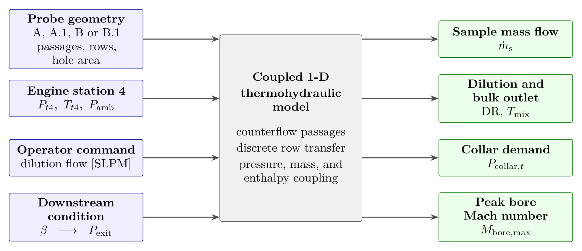
Prototype softwareA steady one-dimensional thermofluid application for designing coaxial dilution sampling probes. It takes a probe geometry, an engine state and a commanded dilution flow. It solves the capture, pressure, mixing and heat-transfer problems together. It returns the sample flow, dilution ratio, supply pressure, outlet temperature and a solution class. I used it to design the probe on the Station 4 sampling apparatus page. It is verified against an independent implementation, but it has no experimental validation.
WhatWhat the software is for
A dilution probe inside a micro-turbojet combustor is a strongly coupled problem. The wall heats the dilution air before it reaches the bore. The bore pressure drop depends on the temperature of the mixed gas. The sample is drawn by a suction margin that is the small difference between two large pressures.
That means no part of the probe can be sized alone. I wrote this application to solve the hydraulic and thermal problems together, quickly enough for design searches that evaluate hundreds of states. Its design results, and the probe they produced, are on the Station 4 sampling apparatus page.
HowInputs
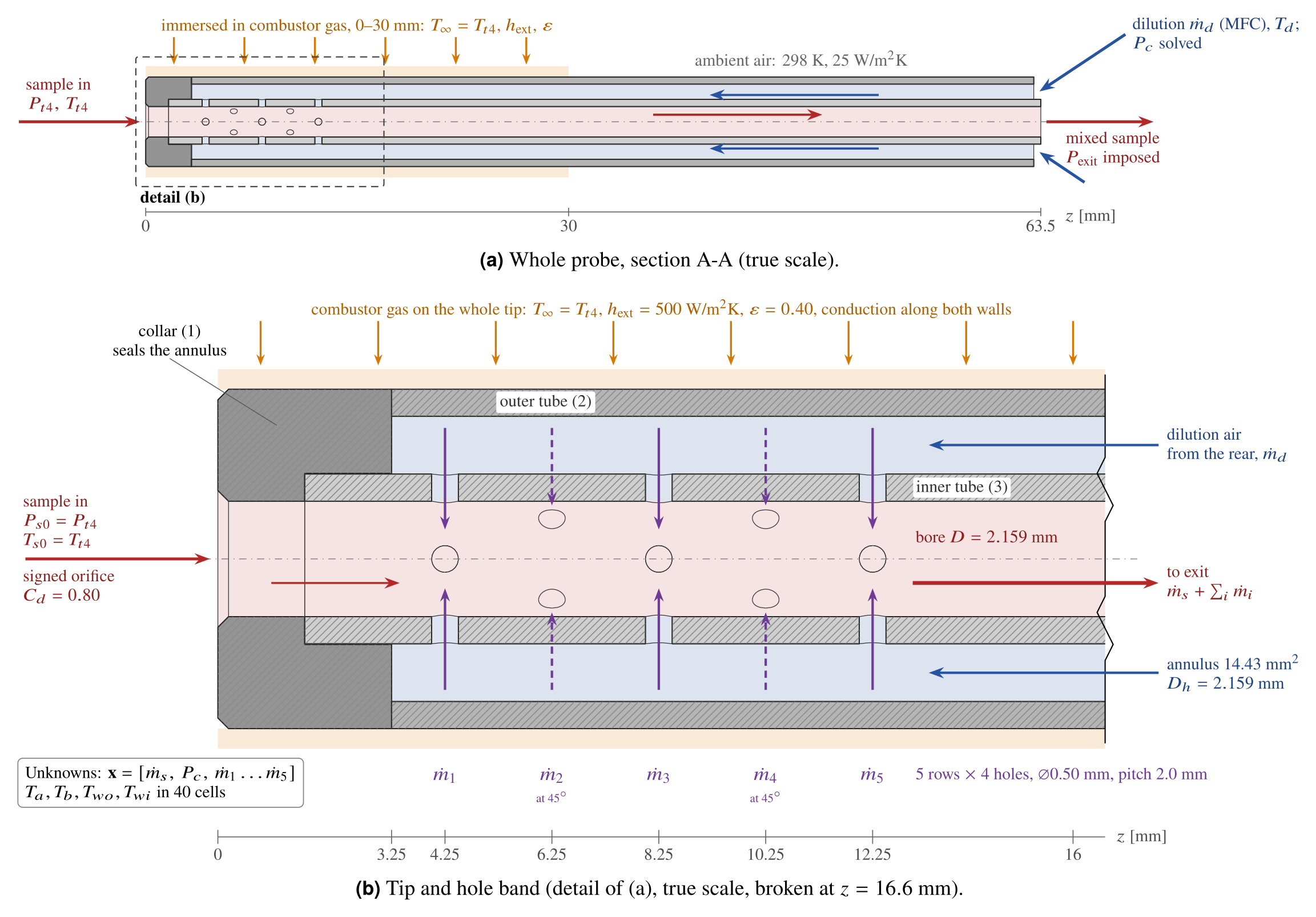
Geometry. A coaxial two-tube probe is defined by its tube diameters and walls, its modeled length and a table of hole rows. The software derives the bore area, the annulus area, the hydraulic diameters and the ratio of hole area to inlet area. The default geometry is the drawn B.1 probe. Geometries from the first (MATLAB) study remain as reference cases.
Engine boundary conditions. The sample reservoir is the combustor total state \((P_{t4},T_{t4})\) with the ambient pressure. Three presets come from steady windows of P200-SX test-cell data. Users can also define their own conditions. The fuel–air ratio of the sample is solved from \(T_{t4}\), assuming complete combustion of Jet A-1.
Installation and heat transfer. The immersed length sees combustor gas at \(T_{t4}\), with a film coefficient and an emissivity. The rest of the probe sees ambient air. The defaults are 30 mm, 500 W/(m²·K) and 0.40.
Dilution command and downstream condition. A mass-flow controller command in SLPM sets the dilution mass flow. The supply pressure that pushes this flow through the probe is an unknown. The static pressure at the bore exit is imposed, as a back-pressure regulator would hold it. In design mode the software solves for that pressure instead.
HowThe coupled calculation
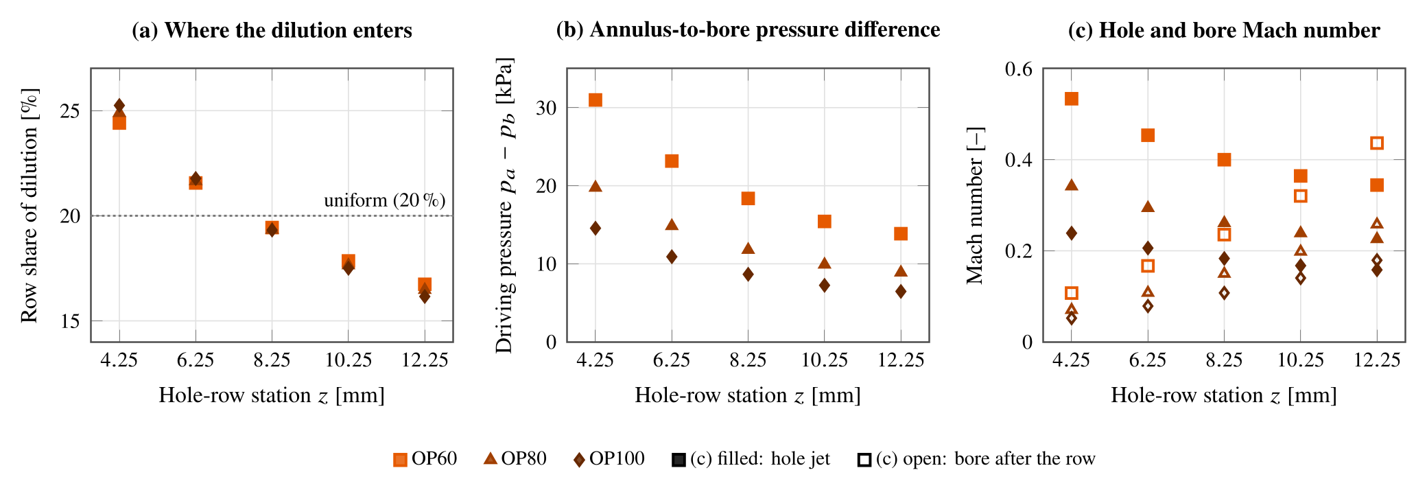
Capture and transfer. The sample inlet and every hole row are compressible orifices. The local pressure difference sets the flow direction, and the gas state comes from the donor side. Row flows are never clipped, so the model can find a reversed row.
\(\Phi\) is the compressible flow function, with a choked branch below the critical pressure ratio. \(C_d\) is 0.70 for the holes and 0.80 for the inlet. DR is the dilution mass flow over the sample mass flow, so the sample is \(1/(1+\mathrm{DR})\) of the outflow.
Pressure along the passages. The bore pressure is marched backward from the exit to the tip. Each segment includes friction and the change in stagnation temperature, and each row adds a momentum jump. The annulus is marched from the supply toward the sealed tip, with partial recovery of dynamic pressure at each row.
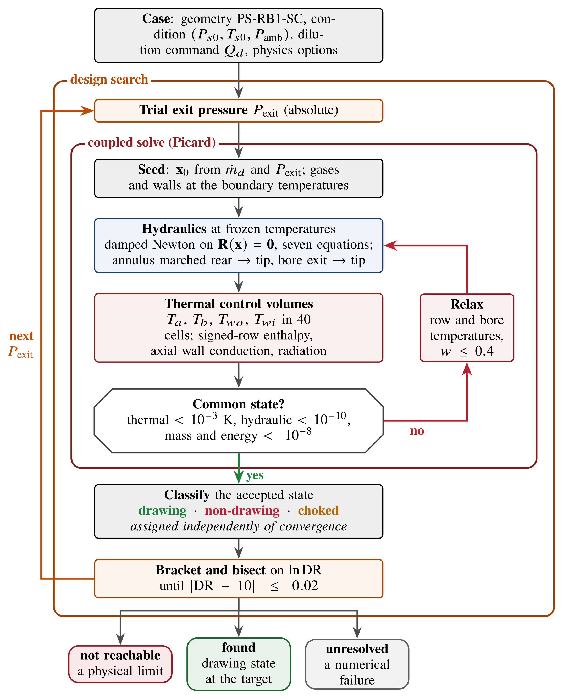
Hydraulic solve. For B.1 the unknowns are the sample flow, the supply pressure and the five row flows. Seven residual equations require the orifice laws to return the assumed flows. A damped Newton method solves them at frozen temperatures.
Mixing and heat transfer. Forty control volumes each carry four temperatures: annulus gas, bore gas, outer wall and inner wall. Heat enters by convection and radiation and conducts along both walls. The gases are balanced in enthalpy, and each row carries enthalpy in its flow direction. Gas properties follow the local dilution fraction.
Coupling and acceptance. A Picard iteration alternates the hydraulic and thermal solves. A state is accepted only when both close at a common state. The residual must be re-evaluated at the new temperatures, and the thermal balance re-solved at that hydraulic state.
ResultsOutputs and solution classes
Each accepted state reports these values:
- the sample mass flow and the dilution ratio
- the dilution supply pressure at the rear of the annulus (the collar pressure in the first version)
- the bulk outlet temperature, and the wall and gas temperatures along the probe
- the suction margin at the tip, the row flows and the Mach numbers.
A separate step classifies every accepted state as drawing, non-drawing or choked. This step does not depend on whether the solver converged. The design search then ends in one of three outcomes:
- Found: a converged drawing state at the target dilution ratio.
- Not reachable: a physical verdict. No exit pressure gives a drawing state at the target.
- Unresolved: a numerical verdict. A solver failure is never read as a physical limit.
The desktop application wraps these services in a stepwise workflow. It covers the study type, geometry, physics options, a pre-run check, the run, results, diagnostics, sensitivity studies and design-review panels. The command-line interface runs the same services.
ResultsHow the results informed the design
The first version compared four probe configurations that split the same cross-section in different ways. That study showed which configuration could reach a dilution ratio of 10 within a realistic dilution supply. It selected configuration B.1.
The second version solved the drawn B.1 geometry and turned the target dilution ratio into a regulator setpoint, with its margin, headroom and sensitivity. The details of both steps are on the Station 4 sampling apparatus page.
ResultsAssumptions and evidence
Verification checks that the equations are solved correctly. It cannot show that they describe the probe. With the baseline closures, the Python version reproduces the MATLAB version to within \(3\times10^{-10}\) in DR. The comparison uses six frozen states of the 32-hole study geometry. A separate first-principles script also checks the drawn-geometry setpoints. That check found an integration error in the bore march, which I corrected.
The main assumptions are these:
- The flow is steady and one-dimensional. The model does not resolve jet penetration, radial mixing or the 45° clocking of alternate rows.
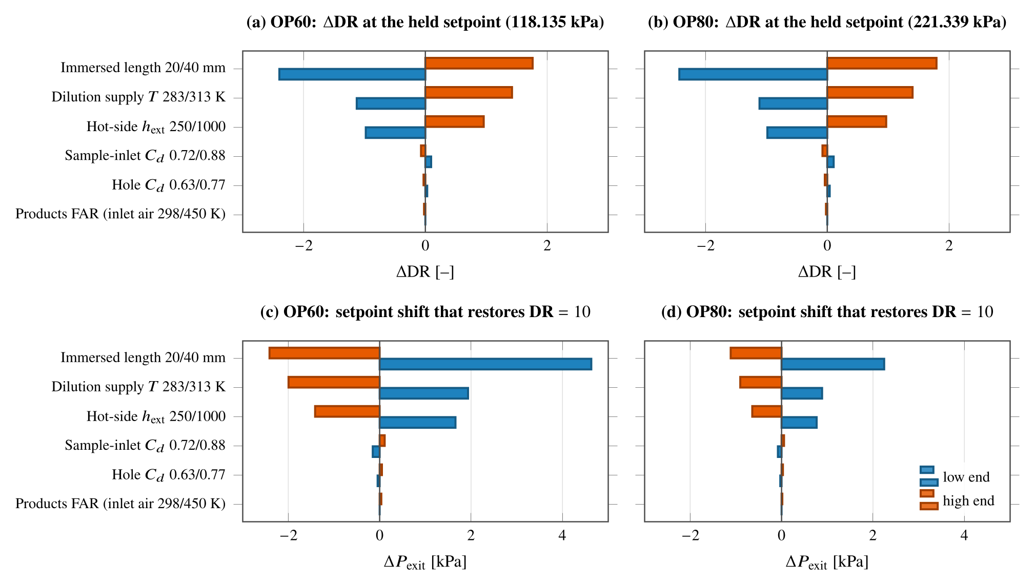
- The discharge coefficients, the annulus recovery coefficient, the hot-side film coefficient, the emissivity and the immersed length are closures or scenario inputs. None is measured on this hardware.
- The engine states come from the P200-SX, and the combustor geometry around the probe comes from hand measurements.
- The bore temperature is a bulk value. It is not evidence of a uniform quench, chemical freeze-out or particle preservation, because the model contains no chemistry and no particle dynamics.
The thermal inputs dominate the sensitivity. Changing the immersed length from 20 to 40 mm moves DR by −2.4 and +1.8 at the held OP60 setpoint. The discharge coefficients move DR by at most 0.10.
There is no experimental validation. No prediction of this software has been compared with a measurement of the B.1 probe.