Wall-Interference Corrections for a Joukowski Airfoil
Personal projectIn MECH 489 Lab 2, my group tested a Joukowski airfoil with a chord close to a third of the wall spacing (c/H = 0.3075). I derived wall corrections for it from first principles, but we never applied them. I came back to my hand notes, checked every step against a panel method with exact walls, found the errors and fixed them.
WhatWhy I came back to this
MECH 489 Lab 2 was a fourth-year undergraduate lab at UBC. We tested a two-dimensional Joukowski airfoil in the Parkinson wind tunnel.
Our model was large for the tunnel. The chord was 0.3075 m and the side walls were 1.0 m apart, so \(c/H=0.3075\). Our lab report named blockage as the main source of error.
While I wrote the report, I derived wall corrections on my own, from first principles. I used a one-dimensional continuity argument for blockage and the method of images for streamline curvature. The group never applied them to the data.
Later I came back to find out if they were right. I checked each step, built a potential-flow benchmark with exact walls, and applied the result to our measurements.
WhatWhat was wrong, and what was right
The short answer is that half of it held up. Here is the full list.
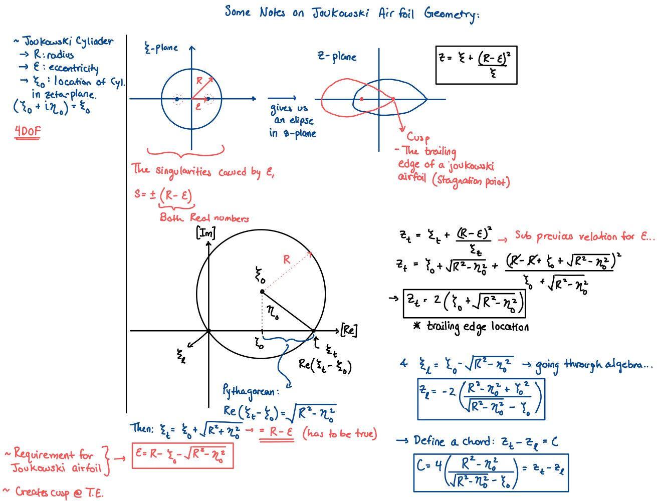
- The Joukowski geometry (page 1) is exact. My chord formula agrees with the numerical chord to 17 parts per million.
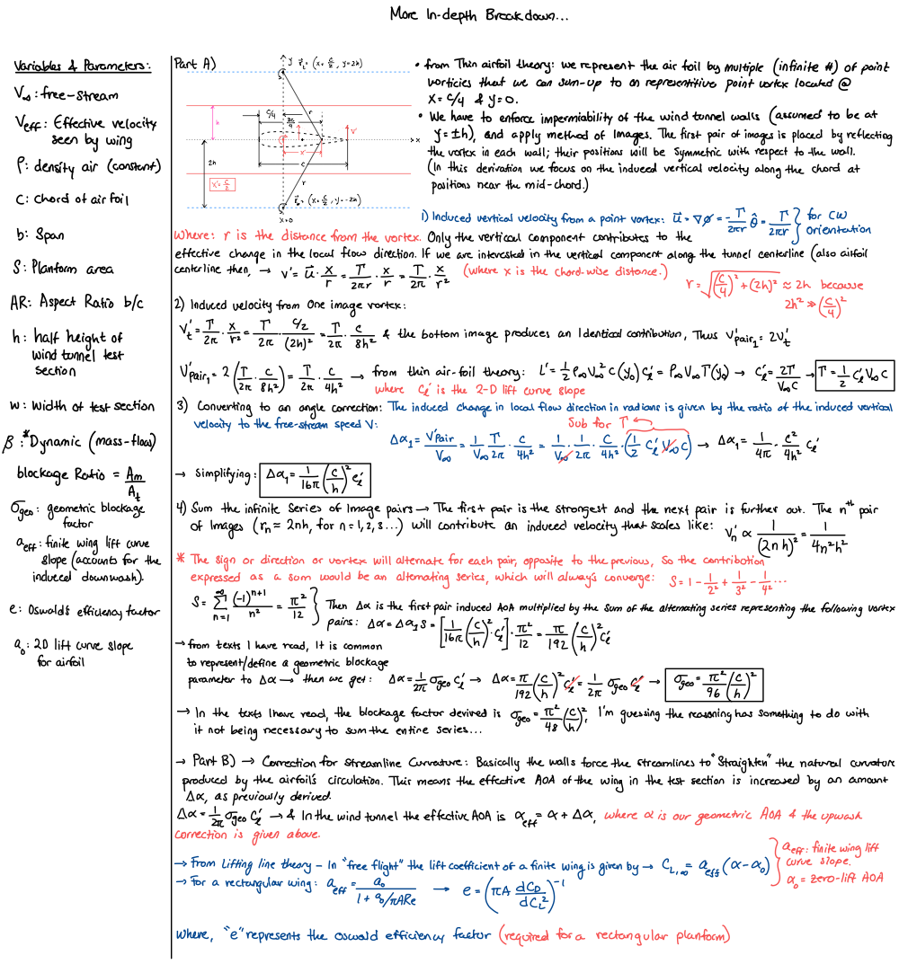
- The curvature correction (page 3) is correct. My factor \(\sigma_{\mathrm{geo}}=(\pi^2/96)(c/h)^2\) is exactly twice the textbook \(\sigma_{\mathrm{AV}}\), because I evaluated the image upwash at the ¾-chord point. A cambered section adds only a small \(2C_m\) term.
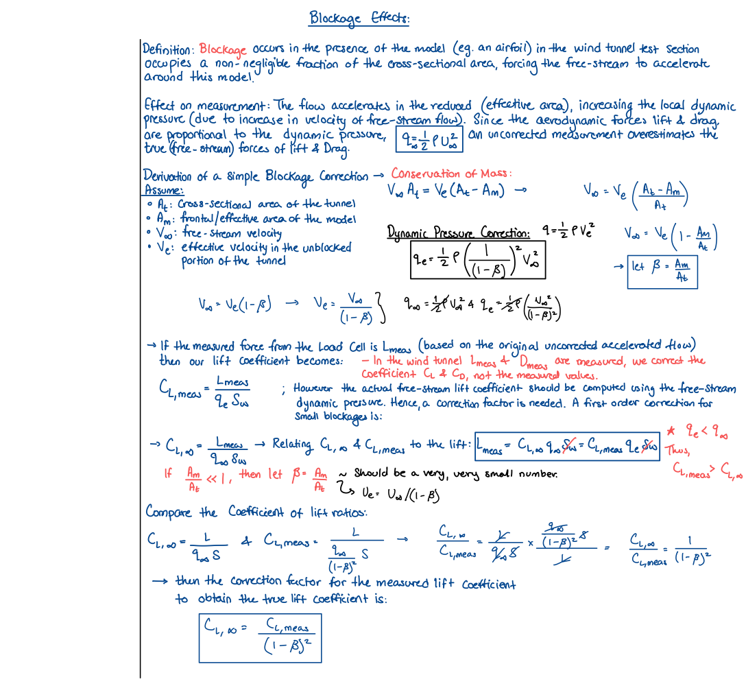
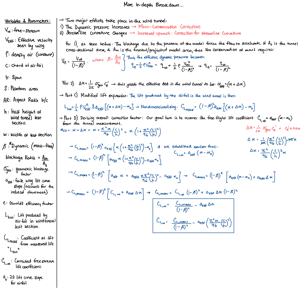
- A sign error (pages 2 and 4). I swapped the labels of the two dynamic pressures. As written, the correction raises \(C_L\) at 8° from 1.175 to 1.296 instead of lowering it. It was a small bookkeeping error with a large effect.
- A model error (pages 2 and 4). The one-dimensional area ratio \(\beta\) is 9 to 19 times the real solid blockage. With the sign fixed, the notes still over-correct by 10.4% in potential flow at 8°.
- The fix. I applied my own method of images to the thickness doublet and to the wake source, and added the \(2C_m\) term. This corrected method leaves −0.1%.
The sign fix alone did not make the notes correct. The bigger error was in the physics of the blockage model. The tool to fix it was already on page 3.
HowThe experiment
The Parkinson wind tunnel at UBC is a closed-circuit facility. Its test section is 0.7 m high, 1.0 m wide and 2.6 m long, with speeds from 5 to 35 m/s [11].
A Betz manometer measures the static-pressure drop across the contraction, upstream of the model. The lab conversion is \(V=4.03\sqrt{h_B}\), with \(V\) in m/s and \(h_B\) in mm of water.
This gives the empty-tunnel reference speed \(V_u\), which the model barely changes. That fact sets the direction of every blockage correction on this page.
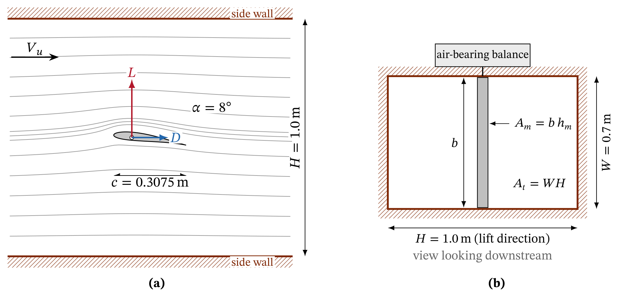
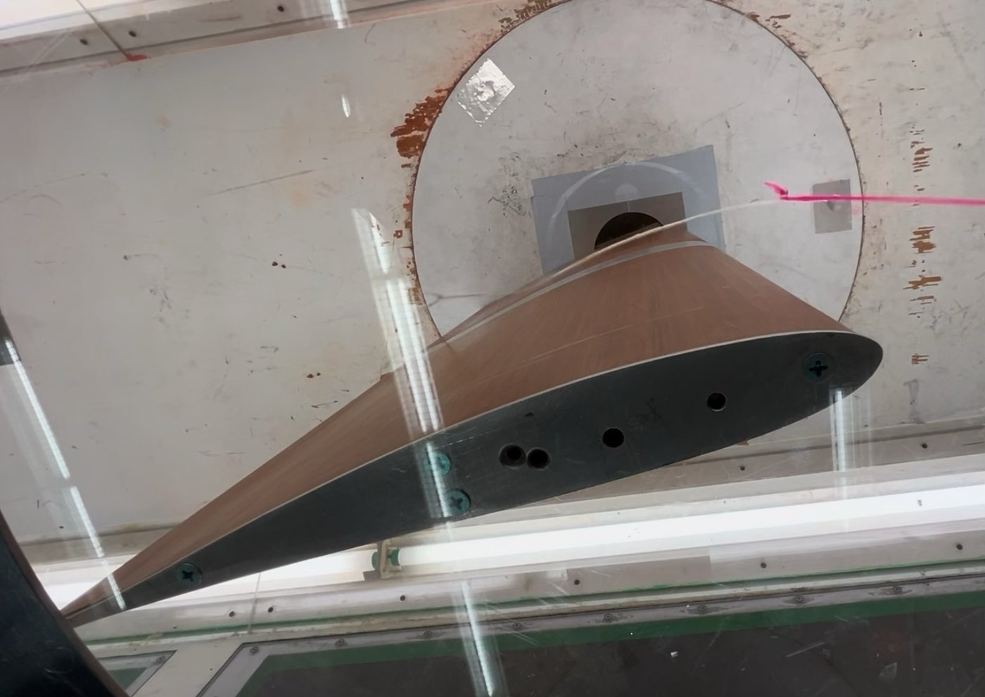
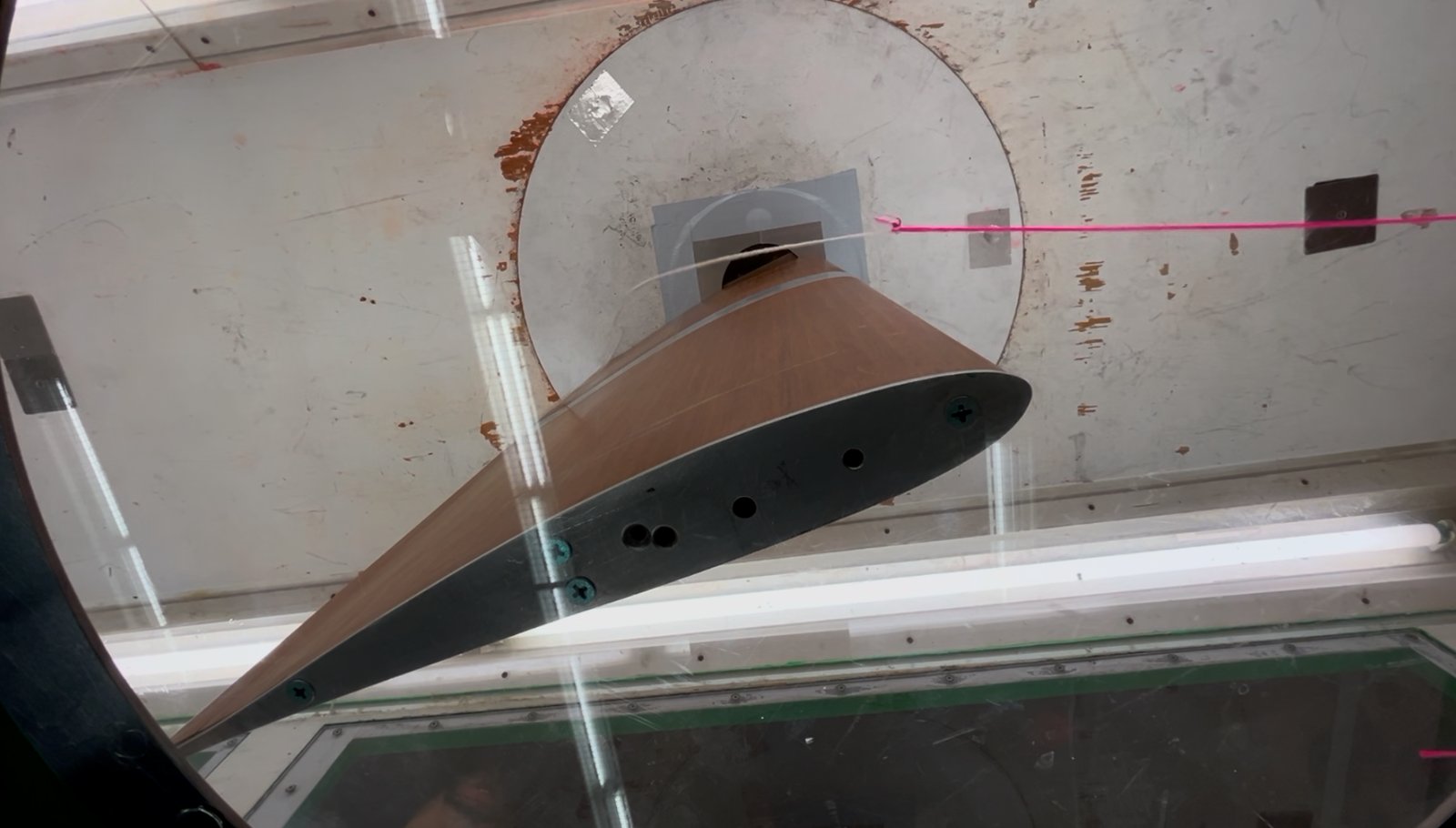
The model has a chord \(c=0.3075\) m and a span \(b=0.6858\) m (27 in). It spans the 0.7 m height of the test section, with a gap of about 7 mm at each end. It hangs from an air-bearing force balance above the ceiling, through a turntable.
Lift therefore acts toward the side walls, and the wall spacing that matters is the width, \(H=1.0\) m. The thickness and camber ratios are \(t/c=0.111\) and \(f/c=0.024\).
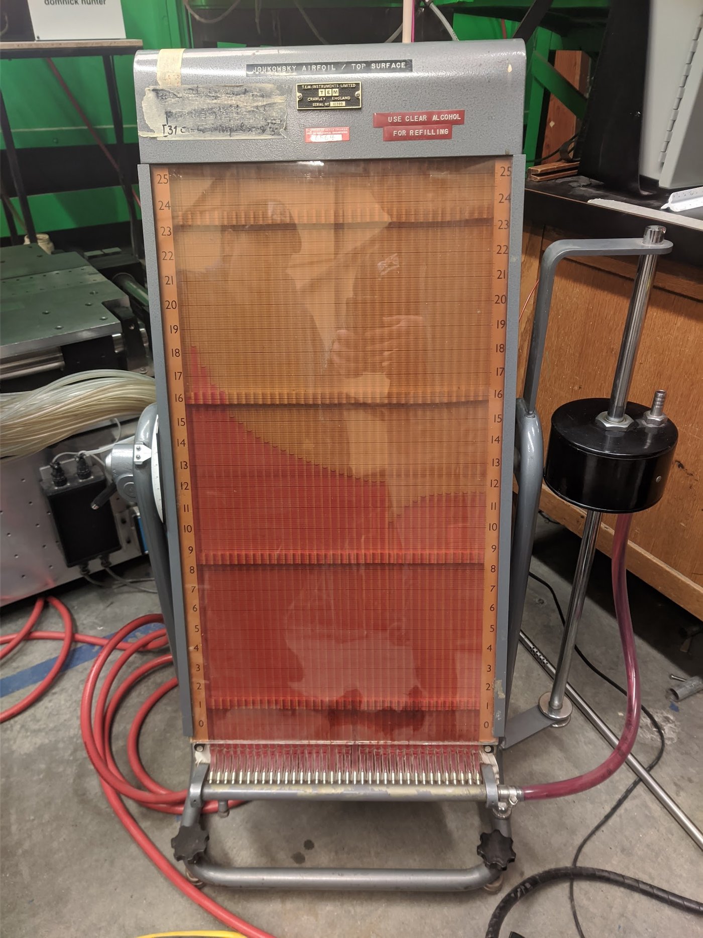
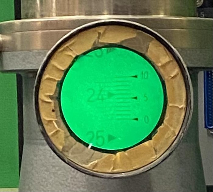
Thirty-six pressure taps, 24 on the upper surface and 12 on the lower surface, connect to a multitube alcohol manometer inclined at 60°.
| Quantity | Symbol | Value |
|---|---|---|
| Test-section width (lift direction) | \(H=2h\) | 1.0 m |
| Test-section height (span direction) | \(W\) | 0.7 m |
| Chord, span, planform area | \(c\), \(b\), \(S\) | 0.3075 m, 0.6858 m, 0.2109 m² |
| Thickness and camber ratios | \(t/c\), \(f/c\) | 0.111, 0.024 |
| Chord and thickness against wall spacing | \(c/H\), \(t/H\) | 0.3075, 0.0341 |
| Frontal-area ratio, −10° to 12° | \(\beta=A_m/A_t\) | 0.034–0.072 |
| Air density, kinematic viscosity | \(\rho\), \(\nu\) | 1.2013 kg/m³, \(1.506\times10^{-5}\) m²/s |
| Reference speed and dynamic pressure (Parts 1–2) | \(V_u\), \(q_u\) | 22.1 m/s, 292.7 Pa |
| Chord Reynolds number (Parts 1–2) | \(Re\) | 4.51 × 10⁵ |
| Chord Reynolds number (Part 3) | \(Re\) | (2.8–5.8) × 10⁵ |
The test had three parts:
- Part 1: lift and drag from −10° to 12° in 2° steps, at \(h_B\approx 30\) mm (\(q_u\approx 293\) Pa)
- Part 2: stall identification at 14° with tufts and smoke, and lift, drag and surface pressures at 8°
- Part 3: lift and drag at 8° for six speeds, \(h_B=11.4\) to 50.4 mm.
I form the uncorrected coefficients with the reference dynamic pressure and the planform area:
The subscript \(u\) means uncorrected. I use the density at the measured room conditions. The original spreadsheet used 1.2 kg/m³, which changes the coefficients by 0.1%.
The balance reports the mean and standard deviation of each force record. The number of samples was not recorded. I take the standard deviation itself as the random uncertainty, which is conservative.
HowJoukowski geometry (notes, page 1)
The Joukowski transformation maps a circle in the \(\zeta\)-plane onto an airfoil in the \(z\)-plane [6, 7]:
Circle radius \(R\) and eccentricity \(\varepsilon\), in the notation of my notes. The mapping is singular where \(\mathrm{d}z/\mathrm{d}\zeta=1-b^2/\zeta^2\) is zero, at \(\zeta=\pm b\).
A circle centered at \(\zeta_0=\xi_0+i\eta_0\) maps to a smooth closed curve, unless it passes through a singular point. If it passes through \(\zeta=+b\), the image has a cusp there. That cusp becomes the trailing edge.
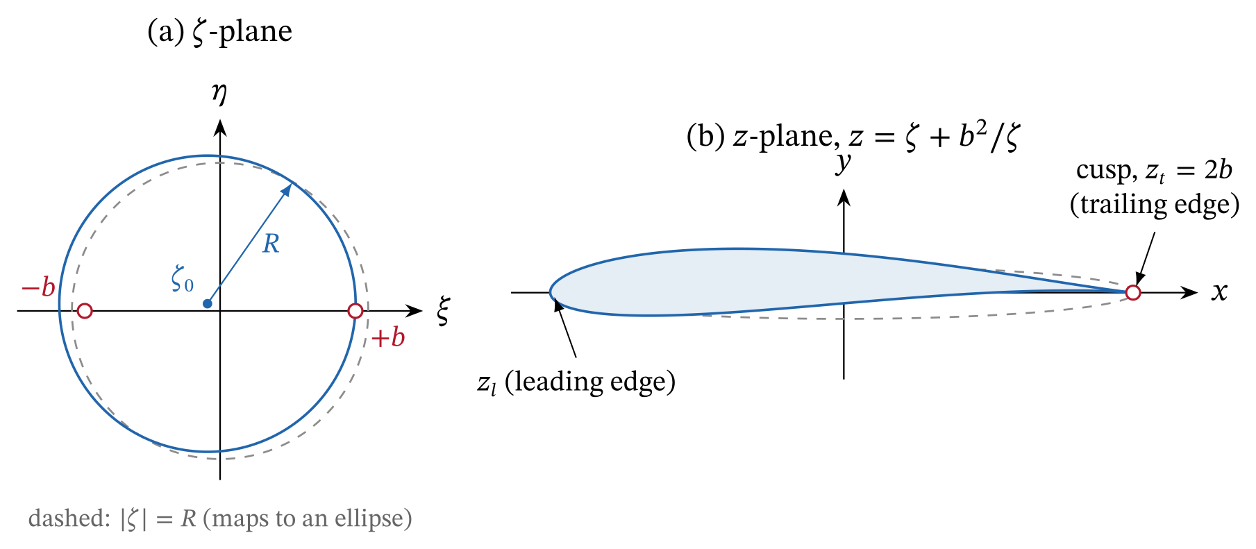
Cusp condition. The circle crosses the real axis at \(\xi_0\pm\sqrt{R^2-\eta_0^2}\). For a cusp, the right-hand crossing must sit on the singular point:
The cusp condition removes one of the four circle parameters \((R,\varepsilon,\xi_0,\eta_0)\), and \(b\) only sets the scale. The two parameters that remain set the thickness and the camber.
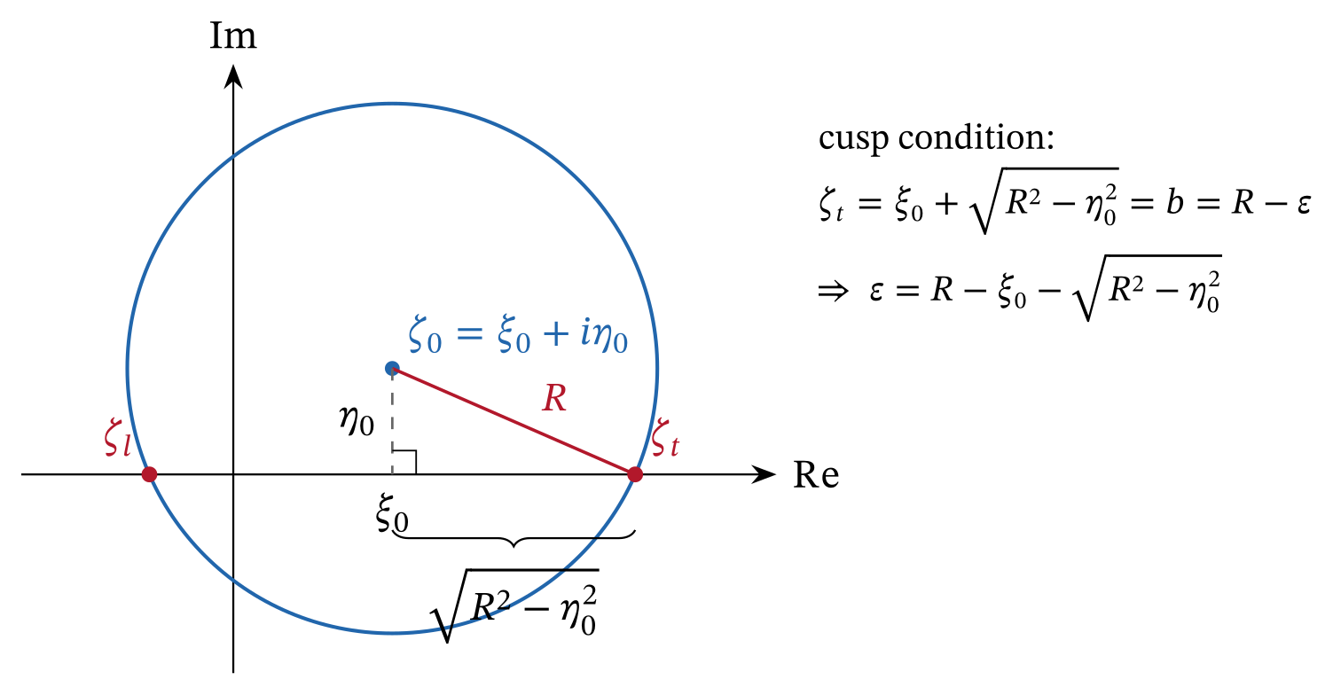
Chord. Substitution of \(\zeta_t=b\) into the mapping gives \(z_t=2b\). The left-hand crossing maps to the leading edge. With \(s=\sqrt{R^2-\eta_0^2}\):
These are the boxed results on page 1 of my notes, and they are correct. Strictly, \(\zeta_l\) maps to the true leading edge only when \(\eta_0=0\). For our model the difference is 17 parts per million of the chord.
Fit to the lab model. With \(b=1\), I solved for \(\xi_0\) and \(\eta_0\) so that the maximum thickness and camber match the lab values. This gives \(\xi_0=-0.0934\), \(\eta_0=0.0533\) and \(R=1.0947\).
The maximum thickness is at \(x/c=0.25\) and the maximum camber at \(x/c=0.51\). The section area is \(0.0673\,c^2\).
Exact potential flow. The Kutta condition at the cusp fixes the circulation. The Kutta–Joukowski theorem then gives the lift:
Incidence \(\alpha\) and zero-lift angle \(\alpha_0\), both from the chord line. For our model, \(\alpha_0=-2.75^\circ\) and the lift-curve slope is 6.820 per radian.
The lab formula \(C_L=2\pi(1+0.77\,t/c)(\alpha+2f/c)\) gives 6.820 per radian and −2.75°. So the classical thickness-and-camber approximation agrees with the exact solution to four significant figures.
Integration of the exact surface pressure gives \(C_{m,c/4}=-0.0765\) at \(\alpha=0\) and \(-0.0806\) at 8°. The balance did not measure pitching moment, so I use these values where a correction needs one.
HowThe corrections as I first derived them (pages 2–4)
This section restates my notes in clean notation. I keep the errors that change the result as written. The next section discusses them.
Blockage by conservation of mass (page 2). Let \(A_t\) be the test-section area and \(A_m\) the frontal area of the model. Mass conservation between an upstream station and the model station gives:
\(V_e\) and \(q_e\) are the speed and dynamic pressure beside the model. I take \(A_m=b\,h_m(\alpha)\), where \(h_m\) is the frontal height of the inclined section. Then \(\beta\) goes from 0.0346 at 0° to 0.0724 at 12°.
The notes then define \(C_{L,\mathrm{meas}}=L/(q_e S)\) and \(C_{L,\infty}=L/(q_\infty S)\). They take the second as the free-air value and conclude:
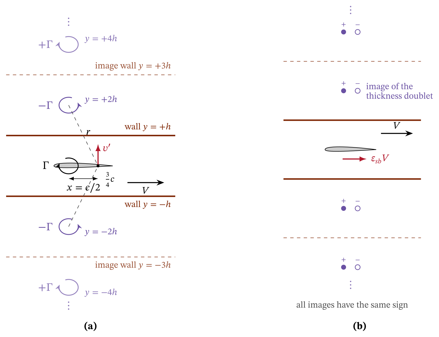
Streamline curvature by the method of images (page 3). Thin-airfoil theory replaces the lifting section with a bound vortex \(\Gamma\) at the quarter chord. The walls are at \(y=\pm h\), with \(H=2h\).
The walls become streamlines if image vortices of alternating sign sit at \(y=\pm 2h,\pm 4h,\dots\) The method slide in the gallery above shows this system. The image upwash grows linearly along the chord, \(v(x)=k\,(x-c/4)\).
Where to evaluate the upwash. Thin-airfoil theory converts a non-uniform upwash into an equivalent change of incidence:
For the linear profile this integral equals \(kc/2V=v(3c/4)/V\). So the ¾-chord point, \(c/2\) behind the vortex, is the exact place to evaluate the upwash for its effect on lift. It is the point I used in the notes.
First pair and full series. For the first image pair, with \(x\ll 2h\) and \(\Gamma=\tfrac12 C_l V c\):
The \(n\)-th pair contributes \((-1)^{n+1}/n^2\) times the first, so the series sums to \(\pi^2/12\):
For our model \(\sigma_{\mathrm{geo}}=0.0389\). The first pair alone would over-estimate the effect by \(12/\pi^2-1=22\%\).
Combined correction (page 4). The model sees the dynamic pressure \(q_e\) and the incidence \(\alpha+\Delta\alpha\). So its lift is \(L=q_eS\,a_{\mathrm{eff}}[(\alpha+\Delta\alpha)-\alpha_0]\).
The notes evaluate \(\Delta\alpha\) with \(C_l'\approx 2\pi\alpha\) and use a finite-wing slope \(a_{\mathrm{eff}}=a_0/[1+a_0/(\pi AR\,e)]\). They arrive at:
ResultsChecking every step
The table lists each step of my notes with an assessment. Most of the derivation holds. The subsections below treat the items that change the result.
| Page | Step as written | Assessment | Correction and comment |
|---|---|---|---|
| 1 | \(\xi_t=\xi_0+\sqrt{R^2+\eta_0^2}\) | Typo | \(\sqrt{R^2-\eta_0^2}\). The boxed cusp condition already uses the minus sign. |
| 1 | \(\varepsilon=R-\xi_0-\sqrt{R^2-\eta_0^2}\), \(z_t=2(\xi_0+\sqrt{R^2-\eta_0^2})\) | Correct | Cusp condition and trailing edge. |
| 1 | \(z_l\) and \(c=4(R^2-\eta_0^2)/(\sqrt{R^2-\eta_0^2}-\xi_0)\) | Correct | Agrees with the numerical chord to 17 ppm. |
| 2 | \(V_e=V_\infty/(1-\beta)\), \(q_e=q_\infty/(1-\beta)^2\) | Correct | One-dimensional continuity. |
| 2 | “\(q_e\lt q_\infty\), thus \(C_{L,\mathrm{meas}}\gt C_{L,\infty}\)” | Sign error | \(q_e\gt q_u\). The two coefficient labels are swapped. |
| 2 | \(C_{L,\infty}=C_{L,\mathrm{meas}}/(1-\beta)^2\) | Sign error | \(C_L=(1-\beta)^2C_{L,u}\). |
| 2, 4 | \(\beta=A_m/A_t\) as the velocity increase at the model | Model too coarse | It counts displacement that also occurs in free air. Images give \(\varepsilon_{sb}=0.0038\), against \(\beta=0.034\)–0.072. |
| 3 | \(r=\sqrt{(c/4)^2+(2h)^2}\approx 2h\) | Typo | \((c/2)^2\): the control point is \(c/2\) behind the vortex. The neglected term is 2.4%. |
| 3 | \(C_l'\) called the “2-D lift-curve slope” | Naming | It is the section lift coefficient, since \(\Gamma=\tfrac12C_lVc\). |
| 3 | \(\Delta\alpha_1\), series \(\pi^2/12\), \(\sigma_{\mathrm{geo}}=(\pi^2/96)(c/h)^2\) | Correct | The exact sum changes the result by −2.7%. |
| 3 | Textbook \(\pi^2/48\) differs because the series need not be summed | Explanation wrong | Textbooks use the full spacing and evaluate the upwash at mid-chord. \(\sigma_{\mathrm{geo}}=2\sigma_{\mathrm{AV}}\). |
| 3 | Bound vortex at \(c/4\) | Assumption | It implies \(C_m=0\). For a cambered section, \(C_l\to C_l+2C_m\). |
| 3, 4 | \(a_{\mathrm{eff}}=a_0/[1+a_0/(\pi AR\,e)]\) | Not applicable | The model spans the test section, so the two-dimensional slope applies. |
| 4 | \(V_e=V_\infty/(1-\beta)^2\) | Typo | \(V_u/(1-\beta)\). The next line for \(q_e\) is correct. |
| 4 | \(C_{L,\mathrm{meas}}=(1-\beta)^2a_{\mathrm{eff}}[(\alpha+\Delta\alpha)-\alpha_0]\) | Sign error | Divide by \((1-\beta)^2\), as on page 2. |
| 4 | \(\Delta\alpha=(\pi^2/96)(c/h)^2\alpha\) from \(C_l'\approx 2\pi\alpha\) | Approximation | It omits \(\alpha_0=-2.75^\circ\). Use the measured \(C_L\). |
| 4 | \(C_{L,\infty}=C_{L,\mathrm{meas}}/(1-\beta)^2-a_{\mathrm{eff}}\Delta\alpha\) | Sign error | \(C_L=(1-\beta)^2C_{L,u}-a\,\Delta\alpha\). |
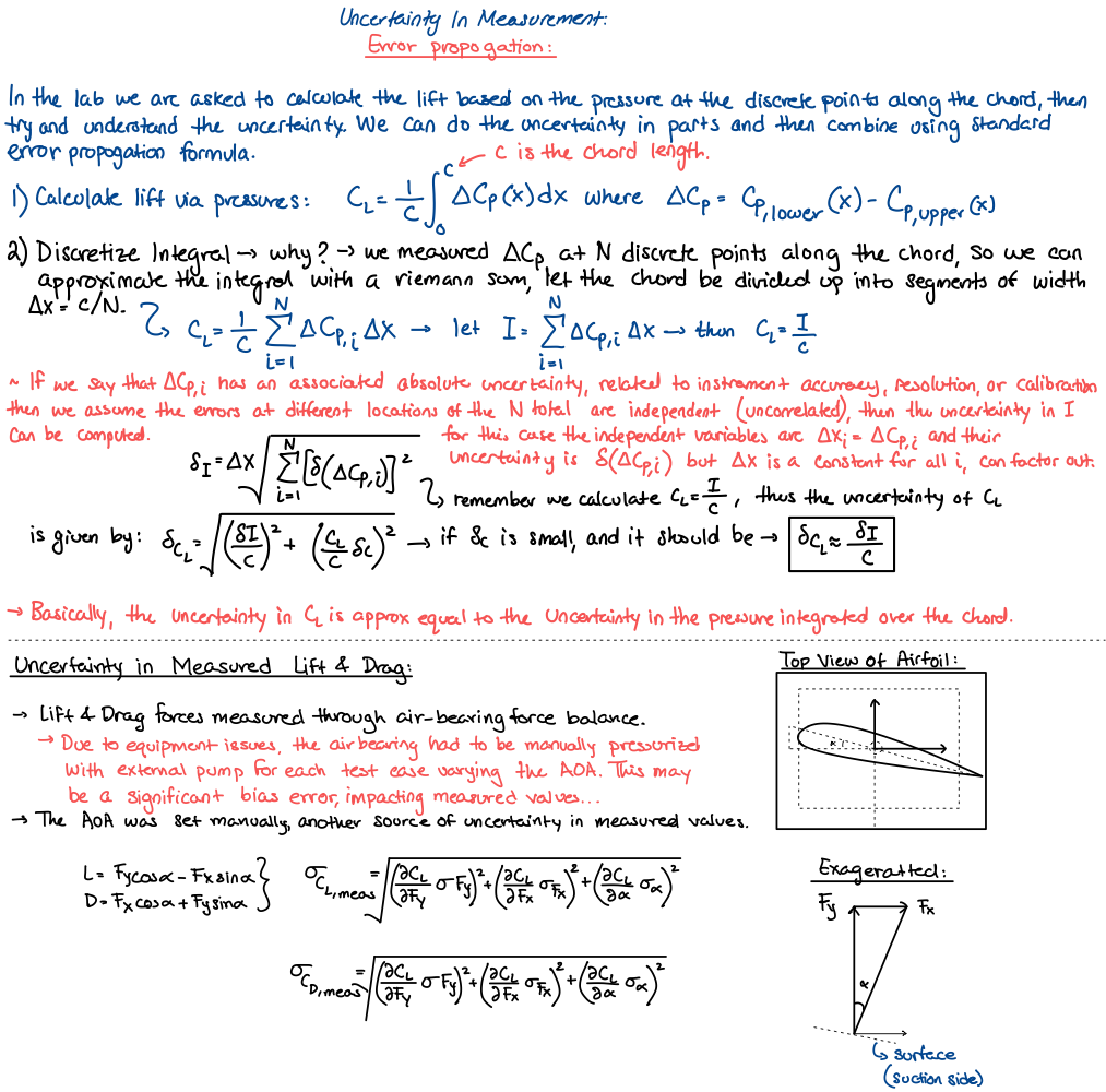
| 5 | \(\delta_I=\Delta x\sqrt{\sum\delta(\Delta C_{p,i})^2}\) | Approximation | The taps are unevenly spaced. Use \(\delta_I=\sqrt{\sum(w_i\,\delta\Delta C_{p,i})^2}\) with trapezoid weights \(w_i\). |
| 5 | \(\sigma_{C_D}\) written with \(\partial C_L/\partial F\) | Typo | \(\partial C_D/\partial F\). |
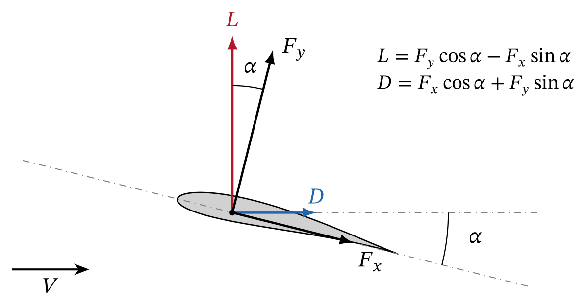
| 5 | \(L=F_y\cos\alpha-F_x\sin\alpha\), \(D=F_x\cos\alpha+F_y\sin\alpha\) | Correct | For a balance in body axes. Then \(\partial C_D/\partial\alpha=C_L\). |
The sign of the blockage correction
The model sees the dynamic pressure \(q_e\), which is larger than \(q_u\). So its lift is \(L=C_Lq_eS\), where \(C_L\) is the free-air coefficient. But the data reduction divides by \(q_u\):
The algebra in my notes is correct, but the labels are swapped. The coefficient normalized by \(q_\infty\) is the one we actually measured. It is not the free-air value.
The physical statement at the top of page 2 is correct: an uncorrected measurement over-estimates lift. The error is only in the bookkeeping after it. The same swap carries into page 4, which corrects to:
Two-dimensional slope \(a\). I compute \(\Delta\alpha\) from the measured lift coefficient, not from \(2\pi\alpha\). The \(2\pi\alpha\) form omits the zero-lift angle and gives no correction at \(\alpha=0\), where \(C_{L,u}=0.445\).
The slope \(a\) falls to zero near stall. I apply the correction as an incidence shift: the point \((\alpha,C_{L,u})\) moves to \(\left(\alpha+\Delta\alpha,\,(1-\beta)^2C_{L,u}\right)\).
Why my curvature factor is twice the textbook one
Page 3 notes that textbooks quote \((\pi^2/48)(c/h)^2\), and I guessed that the series caused the difference. That guess was wrong, but the result was right. The real reason has two parts:
- The textbook factor \(\sigma_{\mathrm{AV}}=(\pi^2/48)(c/H)^2\) uses the full wall spacing \(H=2h\) [1, 4].
- The textbook derivation evaluates the upwash at mid-chord, \(c/4\) behind the vortex. That gives half of the lift effect. It counts the other half as an apparent camber that acts on \(C_L\) directly.
The Allen–Vincenti corrections [1]. \(\varepsilon_{sb}\) and \(\varepsilon_{wb}\) are the solid and wake blockage factors.
At fixed geometric incidence and a slope of \(2\pi\), the two halves add to an incidence shift of \((\sigma_{\mathrm{AV}}/2\pi)(2C_L+4C_m)\). For \(C_m=0\), this equals my \(\sigma_{\mathrm{geo}}C_L/2\pi\), because:
For our model, \(\sigma_{\mathrm{geo}}=0.0389\) and \(\sigma_{\mathrm{AV}}=0.0194\).
My ¾-chord evaluation captures both halves in one incidence correction. It is the classical result in a different but equivalent form.
The exact image sum. The series assumes \(x\ll 2h\). The full sum has a closed form:
At \(x=c/2\) and \(c/H=0.3075\), the cubic term changes the upwash by −2.7%. This is the real higher-order term of the image method, and it is small for our model.
The pitching-moment term
A bound vortex at \(c/4\) puts the center of pressure at the quarter chord. It therefore assumes \(C_m=0\).
For a distributed load \(\gamma(x')\), each element adds image upwash in proportion to \(\gamma(x')(x-x')\). So the total upwash is \(v\propto\Gamma(x-x_{cp})\). It is zero at the center of pressure, not at \(c/4\).
Evaluation at \(\tfrac34 c\), with \(x_{cp}=c/4-C_m c/C_l\), gives:
This is the lift-equivalent form of the Allen–Vincenti incidence correction. For our cambered model \(C_m\approx-0.08\), so the term reduces \(\Delta\alpha\) by about 14% at 8°.
This is a small refinement of the notes.
Solid blockage by the method of images
The continuity estimate assumes that all of the flux the model displaces spreads uniformly over the open area beside it. But a body in free air also displaces flow, and the fluid beside it also accelerates.
That local acceleration exists without walls, so it is already in the free-air coefficients. The walls add only the part that their image system produces. The area ratio therefore counts free-air displacement as wall interference.
The fix uses the same reasoning as page 3. Far from the body, a symmetric thickness distribution acts as a doublet aligned with the stream. Each wall reflects the doublet with the same sign, so the images sit at \(y=\pm H,\pm 2H,\dots\)
An image at distance \(nH\) induces a streamwise velocity \(\mu/(2\pi n^2H^2)\) at the model. The sum over both rows is:
Doublet strength \(\mu\). For an ellipse of thickness ratio \(\tau\) and section area \(A\), \(\mu=VA(1+\tau)\), so \(\varepsilon_{sb}=2\tau(1+\tau)\,\sigma_{\mathrm{AV}}\).
The doublet strength depends on the section shape. Allen and Vincenti give the general form [1]:
Half-thickness \(y_t\) and pressure \(C_p\) on the symmetric thickness form. For an ellipse this reduces to \(\Lambda=2\tau(1+\tau)\).
For a symmetric Joukowski section with \(t/c=0.111\), this gives \(\Lambda=0.193\). My panel method gives 0.190. The ellipse value, 0.247, is larger because an ellipse encloses more area at equal thickness.
The result is \(\varepsilon_{sb}=0.0038\), against \(\beta=0.0346\) to 0.0724 from the area ratio. The difference is structural. The area ratio is first order in \(t/H\), but the image result is second order, \(\varepsilon_{sb}\propto tc/H^2\).
For a streamlined model, the continuity estimate is only an upper bound.
Wake blockage by the method of images
My notes do not include wake blockage, but it follows from the same method.
To the outer flow, the momentum deficit of the wake looks like a source at the model, with strength \(Q=D/(\rho V)=\tfrac12 VcC_D\). Its wall images have the same sign and form a row with spacing \(H\).
The row drives a velocity of \(\pm Q/(2H)\) far downstream and far upstream. The Betz measurement fixes the upstream reference. A uniform flow of \(Q/(2H)\) must therefore be added, which raises the velocity at the model by:
This agrees with the wake term \(\tau c_d\), \(\tau=c/4h\), of Allen and Vincenti [1]. For our data, \(\varepsilon_{wb}\) goes from 0.0018 at 0° to 0.0094 at 12°.
Some later practice uses a coefficient of 1/2 in place of 1/4. I carry that difference as a model uncertainty.
The corrected method
The corrected method combines four parts:
- the corrected sign
- the image solid blockage
- the image wake blockage
- my curvature correction with the \(2C_m\) term.
The drag expression is the standard form [1, 4]. It adds the horizontal buoyancy of the image system to the dynamic-pressure correction.
| Level | Lift coefficient | Incidence | Drag coefficient |
|---|---|---|---|
| Uncorrected | \(C_{L,u}\) | \(\alpha_u\) | \(C_{D,u}\) |
| Continuity, sign corrected (p. 2) | \((1-\beta)^2C_{L,u}\) | \(\alpha_u\) | \((1-\beta)^2C_{D,u}\) |
| Hand notes, sign corrected (pp. 2–4) | \((1-\beta)^2C_{L,u}\) | \(\alpha_u+\sigma_{\mathrm{geo}}C_L/2\pi\) | \((1-\beta)^2C_{D,u}\) |
| Corrected method | \(C_{L,u}/(1+\varepsilon_{sb}+\varepsilon_{wb})^2\) | \(\alpha_u+\sigma_{\mathrm{geo}}(C_L+2C_m)/2\pi\) | \(C_{D,u}(1-3\varepsilon_{sb}-2\varepsilon_{wb})\) |
| Allen–Vincenti [1] | \(C_{L,u}(1-\sigma_{\mathrm{AV}}-2\varepsilon_{sb}-2\varepsilon_{wb})\) | \(\alpha_u+\sigma_{\mathrm{AV}}(C_{L,u}+4C_m)/2\pi\) | \(C_{D,u}(1-3\varepsilon_{sb}-2\varepsilon_{wb})\) |
HowA panel-method benchmark with exact walls
A correction is only as good as its model of the walls. To test each one without experimental noise, I computed the inviscid flow around the real Joukowski section between two walls.
I then applied each correction to these computed “measurements” and compared the result with the exact free-air solution.
Panel method. The solver is a Hess–Smith panel method [7, 8] that I wrote in Python. It uses constant-strength source panels and one vortex strength shared by all panels.
A Kutta condition sets equal tangential velocity on the two trailing-edge panels. The surface carries \(N=400\) panels, cosine-spaced in arc length on each surface.
Channel Green’s function. I did not panel the walls at \(y=\pm H/2\). Instead, every panel influence uses the Green’s function of the channel. A row of singularities with period \(2H\) sums to a \(\coth\) kernel:
Unit source and unit counter-clockwise vortex at \(z_0\), with mirror point \(\bar z_0=x_0+i(H-y_0)\). Source images keep their sign and vortex images alternate, as in the method slide above.
The free-space part of each influence coefficient is integrated analytically. The image part (the kernel minus its free-space term) is smooth on the airfoil, so a six-point Gauss–Legendre rule integrates it.
Validation. I ran four checks:
- The normal velocity on both walls is zero to \(10^{-17}\) for a source and for a vortex.
- For a circular cylinder of radius \(a\), the image-induced velocity at the center approaches the doublet-image value \((\pi^2/3)(a/H)^2\) as \(a/H\to 0\).
- Without walls, the panel lift-curve slope differs from the exact Joukowski value by −3.6% at \(N=400\). Panels on the two surfaces nearly coincide at the cusp.
- The wall effect converges much faster. The ratio of tunnel to free-air lift at 8° is 1.0436 at \(N=100\) and 1.0437 at \(N=800\).
Because of the slope error, I use the panel method only for the wall increment. I scale it by the slope ratio \(k=1.038\) and add it to the exact free-air solution:
What the walls do at the model
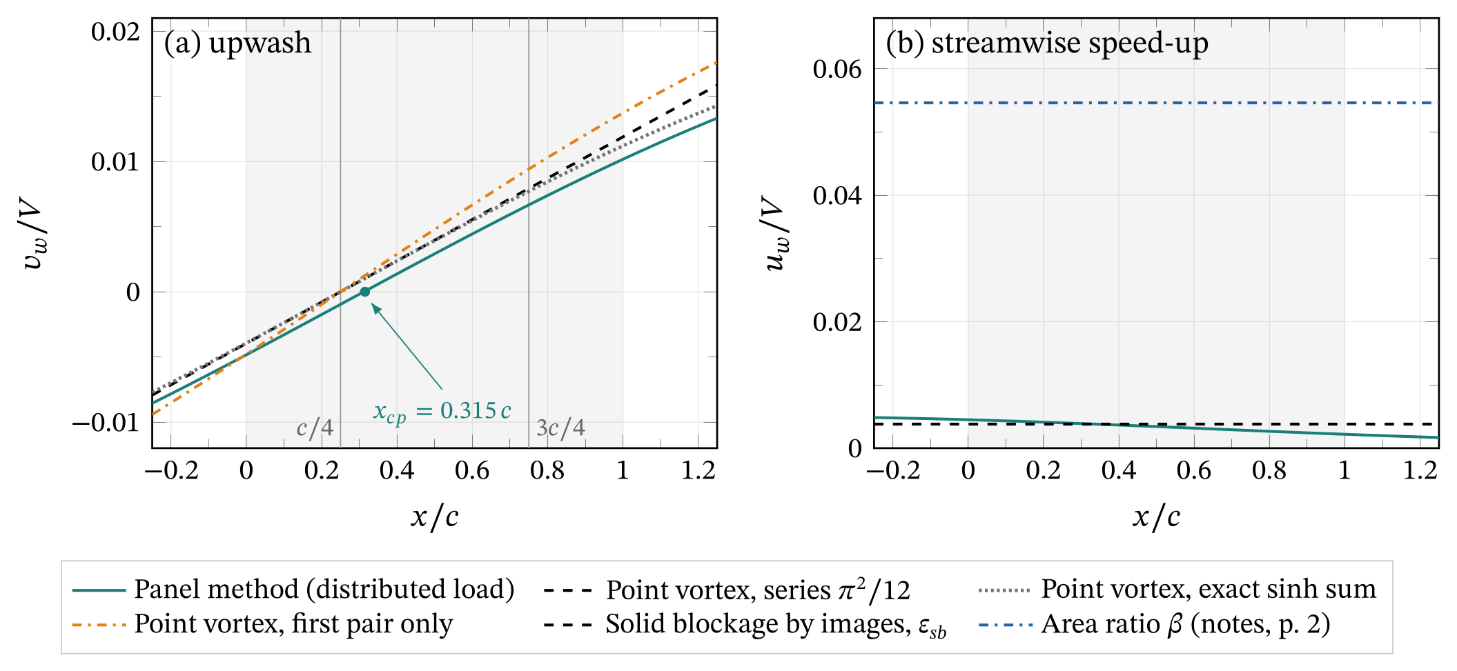
- Upwash. At the ¾-chord point the panel method gives \(v_w/V=0.0067\). The point vortex gives 0.0079 with the \(\pi^2/12\) series, 0.0077 with the exact sinh sum and 0.0094 with the first pair alone.
- Most of the difference between the panel and the point vortex comes from the center of pressure at \(0.315\,c\). This is the pitching-moment effect.
- Speed-up. The panel method gives \(u_w/V\approx0.0034\) along the chord. This is close to the image estimate \(\varepsilon_{sb}=0.0038\) and far below the area ratio \(\beta=0.0546\).
How accurate is each correction?
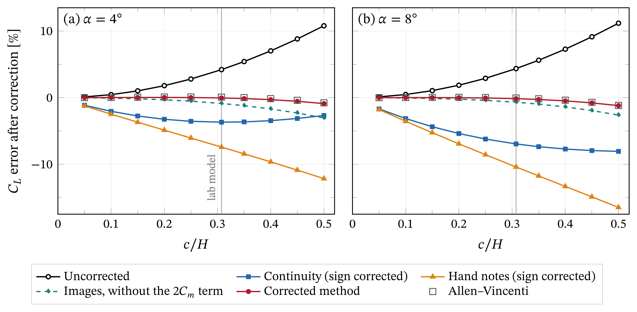
In potential flow at \(c/H=0.3075\), the walls raise the lift by +4.2% at 4° and by +4.4% at 8°. The result slide in the gallery above shows the error left after each correction, for \(0.05\le c/H\le 0.5\).
At the lab value of \(c/H\) and \(\alpha=8^\circ\):
- the continuity correction over-corrects to −7.0%
- my hand-notes set over-corrects further, to −10.4%, because a correct curvature term adds to an excessive blockage term
- image blockage without the \(2C_m\) term leaves −0.7%
- the corrected method leaves −0.1%, the same as Allen–Vincenti (−0.1%).
My curvature derivation is therefore sound. Nearly all of the error in the original set comes from the area-ratio blockage. The corrected method and Allen–Vincenti stay within 1.2% of the free-air lift up to \(c/H=0.5\).
ResultsCorrected results for our data
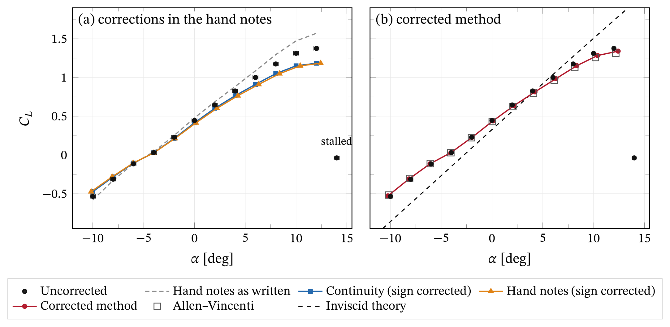
Lift. The 14° point is stalled (\(C_{L,u}=-0.038\), \(C_{D,u}=0.189\)). None of the corrections is valid for separated flow [9], so I show it uncorrected.
- As written, page 4 raises \(C_L\), for example from 1.175 to 1.296 at 8°. This shows the effect of the swapped labels.
- With the sign corrected, the continuity correction and the hand-notes set remove 7 to 14% of the lift. At 8° the continuity correction gives \(C_L=1.050\), and the hand-notes set gives the same value at \(\alpha=8^\circ+0.37^\circ\).
- The corrected method gives \(C_L=1.153\) at \(\alpha=8^\circ+0.35^\circ\). Allen–Vincenti gives 1.130 at \(8^\circ+0.15^\circ\). At the same incidence, the two differ by 0.0049 in \(C_L\).
| \(\alpha_u\) | Uncorrected \(C_{L,u}\) | Continuity \(C_L\) | Hand notes \((\Delta\alpha,\ C_L)\) | Corrected method \((\Delta\alpha,\ C_L)\) | Allen–Vincenti \((\Delta\alpha,\ C_L)\) | Inviscid \(C_l\) |
|---|---|---|---|---|---|---|
| −10° | −0.536 | −0.474 | (−0.17°, −0.474) | (−0.24°, −0.529) | (−0.15°, −0.518) | −0.862 |
| 0° | 0.445 | 0.415 | (0.15°, 0.415) | (0.10°, 0.440) | (0.02°, 0.431) | 0.327 |
| 8° | 1.175 | 1.050 | (0.37°, 1.050) | (0.35°, 1.153) | (0.15°, 1.130) | 1.273 |
| 12° | 1.376 | 1.184 | (0.42°, 1.184) | (0.42°, 1.341) | (0.19°, 1.313) | 1.738 |
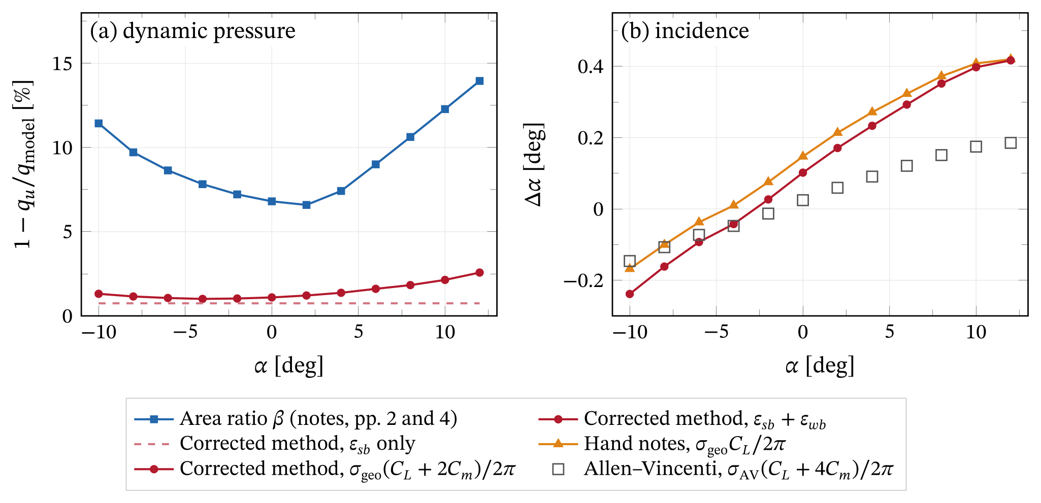
Fig. 9 separates the contributions. The area ratio follows the frontal height of the model, so it grows on both sides of \(\alpha\approx-2^\circ\).
In the corrected method, the constant solid blockage sets the dynamic-pressure correction at low incidence. Wake blockage takes over at high incidence.
The incidence shifts of the hand-notes set and the corrected method differ only through the \(2C_m\) term. It matters most near zero lift, where \(C_m\) is a large fraction of \(C_L\).
Lift-curve slope and zero-lift angle
The table lists linear fits over \(-8^\circ\le\alpha\le 6^\circ\). Every correction lowers the slope, because wall interference raises the apparent slope.
The uncorrected slope is already 0.80 of the inviscid value. After correction it is 0.76. Wall interference cannot explain the low measured slope. The correction widens the gap.
A boundary layer typically lowers the inviscid slope by 5–10% at this Reynolds number. The rest must come from the installation. I see two candidates:
- leakage through the 7 mm end gaps, which acts as a tip loss
- the uncalibrated balance.
Allen and Vincenti traced a similar slope deficit in their own large-chord tests to leakage through end gaps [1].
The zero-lift angle is about −4.6° at every level, against −2.75° from theory. A constant offset in the incidence reference or a slightly deflected trailing-edge flap would explain this. The data cannot tell them apart.
| Level | Slope [rad⁻¹] | Slope / inviscid | \(\alpha_0\) [deg] |
|---|---|---|---|
| Inviscid Joukowski | 6.820 | 1 | −2.75 |
| Uncorrected | 5.45 | 0.80 | −4.61 |
| Continuity (sign corrected) | 4.99 | 0.73 | −4.65 |
| Hand notes (sign corrected) | 4.84 | 0.71 | −4.65 |
| Corrected method | 5.20 | 0.76 | −4.66 |
| Allen–Vincenti | 5.18 | 0.76 | −4.67 |
Drag and lift-to-drag ratio
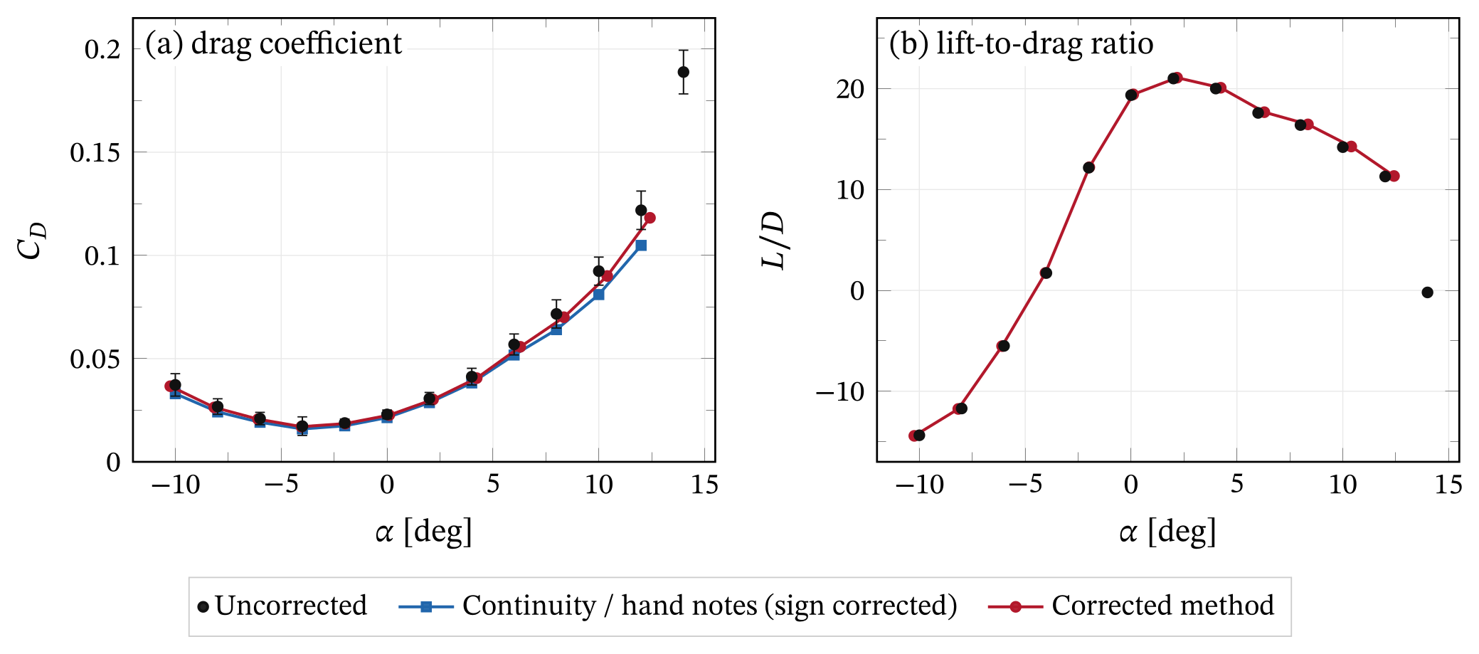
The corrected method lowers the drag by 1.5 to 3% (3.0% at 12°). The continuity correction removes up to 14.0%.
The drag error bars include the body-axis term from page 5 of my notes. At 8°, an incidence error of 0.25° moves 0.0051 of lift into drag. That is 7% of \(C_D\), more than the drag correction itself.
The maximum lift-to-drag ratio is about 21 at \(\alpha\approx 2^\circ\), before and after correction.
Reynolds-number sweep
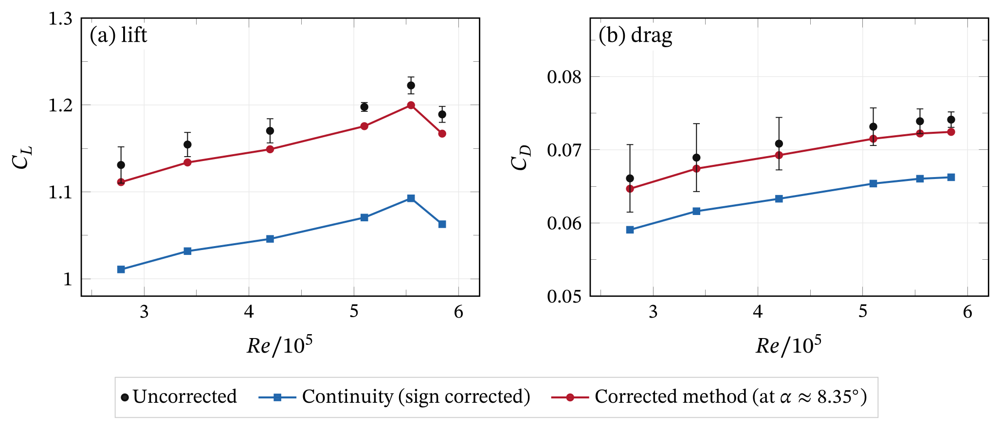
In Part 3 the Reynolds number goes from \(2.8\times10^5\) to \(5.8\times10^5\). Over this range \(C_{L,u}\) rises from 1.131 to a peak of 1.222 at \(Re=5.5\times10^5\), then falls to 1.189.
Over the same range, \(C_{D,u}\) rises from 0.0661 to 0.0741. The corrections depend mostly on geometry, with \(C_D\) only in the wake term. They shift both curves almost uniformly and keep the trends.
A drag coefficient that increases with Reynolds number is unusual for an attached airfoil. Together with the slope deficit, it points to balance behavior rather than flow physics. The data cannot confirm this.
Surface pressure at α = 8°
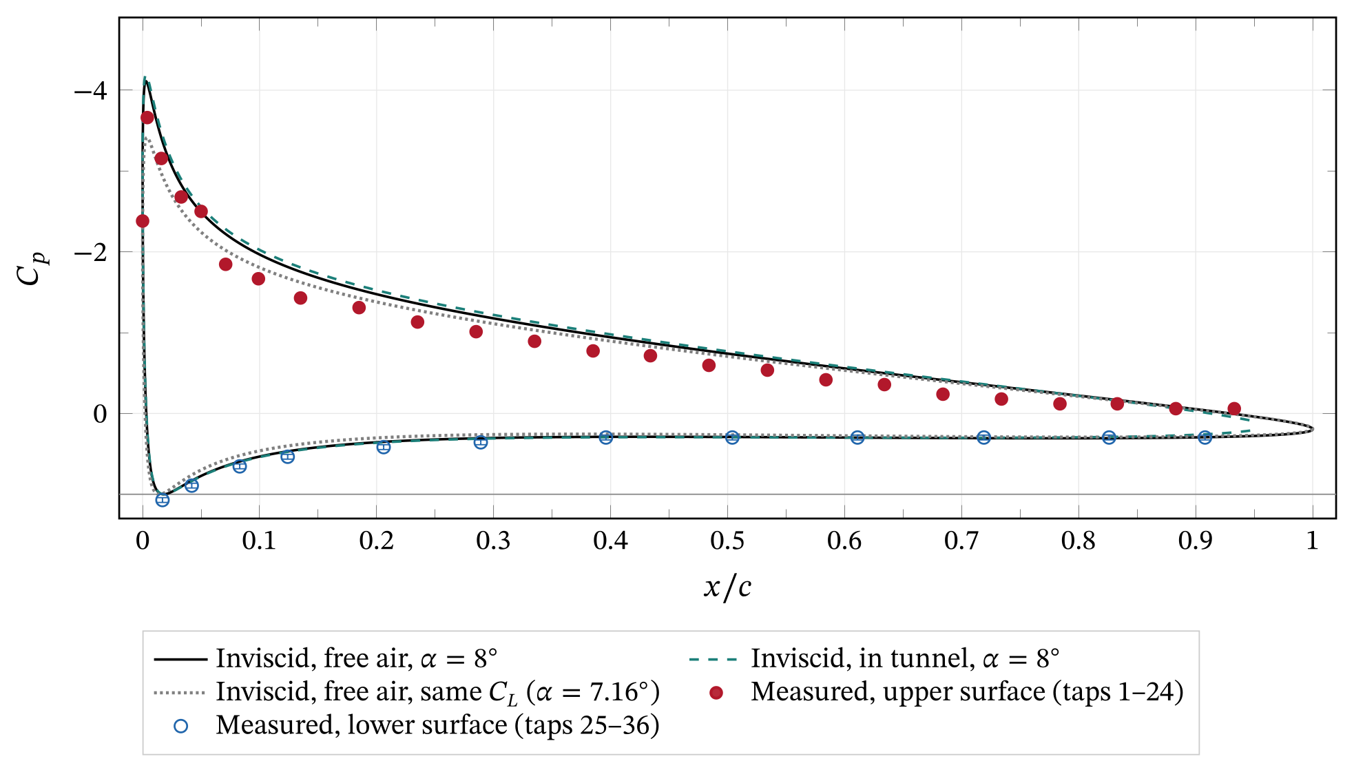
Conversion. I convert each tube reading \(h_i\), in inches along the inclined bank, to a pressure coefficient:
Wind-off level \(h_0=12.1\) in, bank inclination \(\theta_m=60^\circ\) and alcohol density \(\rho_m\). I assume a specific gravity of \(0.81\pm0.02\).
The stagnation tap reads \(C_p=1.07\). A static reference depressed by blockage would explain at most \((1+\varepsilon)^2-1\approx 2\%\) of the excess. The fluid-density uncertainty covers the rest.
Tap positions. The spreadsheet lists 23 upper and 13 lower tap positions, but the report states 24 and 12. With the spreadsheet order, the lower tap at \(x/c=0.017\) reads \(C_p\approx 0\).
But the exact solution puts the stagnation point at \(x/c=1.8\%\) on the lower surface, where \(C_p\) should be close to one. The upper list also has a single 10% gap in an otherwise 5% spacing.
I therefore insert an upper tap at \(x/c=0.484\) and assign tubes 25–36 to the lower stations from 0.017 to 0.908. With this mapping, the stagnation tap is at \(x/c=0.017\).
The upper readings near the trailing edge then also follow one smooth trend.
Integration. The trapezoidal rule on each surface gives \(C_n=1.102\) and \(C_a=-0.168\). The axial force uses the surface slopes of the fitted geometry.
The lift is then \(C_l=C_n\cos\alpha-C_a\sin\alpha=1.114\). This is −5.2% below the balance value of 1.175. The spreadsheet order would give 1.170.
The taps under-resolve the suction peak, so the integral is biased low.
The original value. Our report quoted \(C_L=1.33\) from the pressures, close to the theory line. That agreement was a coincidence.
The spreadsheet divided readings in inches by \(q_uS\) in newtons, used \(\Delta x\) in percent of chord, and integrated in tube order. The lower surface therefore entered with the wrong sign, and two wrap-around segments were included.
With consistent units and signs, the pressure lift agrees with the balance to about 5%.
ResultsUncertainty
The uncertainty analysis follows page 5 of my notes and standard first-order propagation [10]. These are the main contributions at \(\alpha=8^\circ\):
- Random. Fluctuation of the balance record dominates the vertical error bars. The Betz reading resolution of ±0.05 mm adds 0.2%.
- Incidence. The turntable setting accuracy is not documented, so I assume ±0.25°. Along the lift curve this is ±0.024 in \(C_L\), the largest single term.
- Body axes. If the balance axes turn with the model, an incidence error also moves lift into drag (Fig. 13).
- Correction model. A ±5% change in the published wall spacing changes the corrected \(C_L\) by ±0.0047. A wake coefficient of 1/2 instead of 1/4 lowers \(C_L\) by a further 0.0121 at 8° and 0.0237 at 12°.
- Balance calibration. A portable compressor supplied the air bearing, and the balance could not be calibrated. The data cannot quantify this bias. It may be the largest error in the force measurements.
For the pressure integral, the reading resolution propagates with the trapezoidal weights:
The fluid density adds ±0.027. The workbook also records a bank angle of 70° next to the 60° in the report. A 70° bank would raise \(C_n\) to 1.195.
| Quantity | Source | Magnitude |
|---|---|---|
| \(C_L\) (balance) | Balance fluctuation (1σ) | ±0.0138 |
| Betz reading, ±0.05 mm | ±0.0020 | |
| Incidence, ±0.25° (along the lift curve) | ±0.024 | |
| Wall spacing, H ± 5% | ±0.0047 | |
| Wake-blockage coefficient, 1/4 vs 1/2 | −0.0121 | |
| Correction model (corrected method vs Allen–Vincenti) | 0.0049 | |
| Balance calibration | Not quantified | |
| \(C_D\) (balance) | Incidence, ±0.25°, body axes (\(C_L\,\delta\alpha\)) | ±0.0051 (7%) |
| \(C_n\) (pressure) | Reading, ±0.05 in, trapezoidal weights | ±0.011 |
| Fluid specific gravity, 0.81 ± 0.02 | ±0.027 | |
| Bank angle, 60° vs 70° | +0.093 | |
| Tap positions (report vs spreadsheet) | +0.055 | |
| Suction-peak resolution | Biased low, not quantified |
NotesThe original hand notes
These five pages formed the appendix of our lab report. I show them unchanged. The check table above lists every correction.
DiscussionWhat I take from this
Was my derivation correct? For streamline curvature, yes. The image method, the ¾-chord point and the alternating series are all correct. The Joukowski geometry is exact.
For blockage, two things went wrong. The first was bookkeeping. I swapped the labels of the two dynamic pressures, so the formula moves the data the wrong way. It was a small error with a large effect, and easy to fix.
The second was physics. The one-dimensional area ratio treats all displaced flux as wall interference. It over-predicts solid blockage by an order of magnitude, and it grows with the frontal height of the inclined model.
Fixing the sign alone is not enough, because the sign-fixed set still over-corrects by 10.4%. The fix was the method of images, which I had already used on page 3.
I like that the fix was already in my own notes. I only had to point it at the thickness and the wake too.
When the area ratio is useful. It remains an upper bound. For a bluff or fully stalled model, the wake fills a large part of the test section and the flow approaches the one-dimensional picture. Maskell’s method treats that case [9].
Practical guidance for this tunnel. For an airfoil of this size in the Parkinson tunnel, the walls raise the measured lift coefficient by 1–3%. They raise the effective incidence by up to about 0.4°.
The corrected method or the Allen–Vincenti set removes this to better than 1%. Both fit in a lab spreadsheet. The larger problems in this data set are the incidence reference, the balance calibration and the end gaps.
Limitations. The panel benchmark is inviscid, so it cannot test the wake term or separated flow. The pitching moment comes from theory, because the balance did not measure it. The wall spacing comes from published facility data.
Reproducibility. My Python scripts produce every number and plot on this page. The write-up reads all values from a generated file, so I typed none of them by hand.
References
- [1]H. J. Allen and W. G. Vincenti, “Wall interference in a two-dimensional-flow wind tunnel, with consideration of the effect of compressibility,” NACA Report 782, 1944.
- [2]H. Glauert, “Wind tunnel interference on wings, bodies and airscrews,” ARC R&M 1566, 1933.
- [3]A. Thom, “Blockage corrections in a closed high-speed tunnel,” ARC R&M 2033, 1943.
- [4]J. B. Barlow, W. H. Rae and A. Pope, Low-Speed Wind Tunnel Testing, 3rd ed., Wiley, 1999.
- [5]B. F. R. Ewald (ed.), Wind Tunnel Wall Correction, AGARDograph 336, AGARD, 1998.
- [6]J. D. Anderson, Fundamentals of Aerodynamics, 6th ed., McGraw-Hill, 2017.
- [7]J. Katz and A. Plotkin, Low-Speed Aerodynamics, 2nd ed., Cambridge University Press, 2001.
- [8]J. L. Hess and A. M. O. Smith, “Calculation of potential flow about arbitrary bodies,” Progress in Aerospace Sciences 8, 1–138, 1967.
- [9]E. C. Maskell, “A theory of the blockage effects on bluff bodies and stalled wings in a closed wind tunnel,” ARC R&M 3400, 1963.
- [10]H. W. Coleman and W. G. Steele, Experimentation, Validation, and Uncertainty Analysis for Engineers, 4th ed., Wiley, 2018.
- [11]UBC Mechanical Engineering Aerolab, “Facilities: Parkinson Wind Tunnel,” mech.ubc.ca/aerolab/facilities, accessed October 2026.