MECH 477: F100-PW-100 Thermodynamic Cycle Analysis
Course projectAn individual course project in MECH 477 (aerospace propulsion). I wrote a zero-dimensional cycle model of the F-15’s low-bypass afterburning turbofan (BPR 0.69, OPR 24.1, TIT 1680 K). It marches through the engine station by station, with temperature-dependent gas properties, polytropic efficiencies, mixing and a choked convergent nozzle.
WhatModeling a fighter engine from first principles
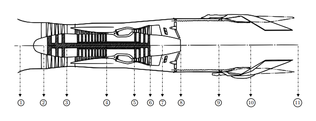
The Pratt & Whitney F100-PW-100 powers the F-15. It is a two-spool, low-bypass turbofan. Its bypass and core streams mix before an afterburner and the nozzle.
The goal was to predict thrust and specific fuel consumption at the on-design, sea-level static point from component physics. The inputs are the values in the course handout. A second goal was to find which parameters have the largest effect on performance.
HowStation-by-station cycle analysis
The model groups the real components into a reduced set. The low- and high-pressure compressors become one effective compressor. The high- and low-pressure turbines become one effective turbine, which drives both the fan and the compressor. The report states that this grouping does not change the station-level conservation equations.
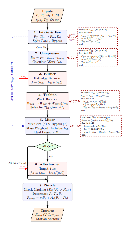
The MATLAB model then marches through the engine one station at a time:
- The fan, the compressor and the turbine use polytropic efficiencies, so pressure ratio and efficiency stay consistent across operating points.
- Specific heat changes with temperature, from polynomial fits.
- The burner and the afterburner use an enthalpy balance on the fuel.
- The single turbine supplies the fan and compressor work, divided by the mechanical efficiency.
- The mixer uses an enthalpy balance for temperature. For pressure, it uses a mass-weighted average with a loss factor, or a 1-D momentum balance at matched static pressure in the sweeps.
Station numbers follow the report: 3 is the fan exit, 4 the compressor exit, 5 the turbine inlet and 6 the turbine exit. The compressor temperature ratio follows from the pressure ratio and the polytropic efficiency \(\eta_{p,c}\). The burner energy balance gives the fuel flow. The solver uses the simpler form \(f\approx(h_{05}-h_{04})/(\eta_bQ_{\mathrm{LHV}})\), which drops a small term. The last relation is the single turbine work balance.
At sea-level static conditions the inlet momentum is negligible, so the net thrust equals the gross jet thrust. The pressure term comes from the choked nozzle. SFC uses the main-burner and afterburner fuel flows.
ResultsClose to the published ratings at one point
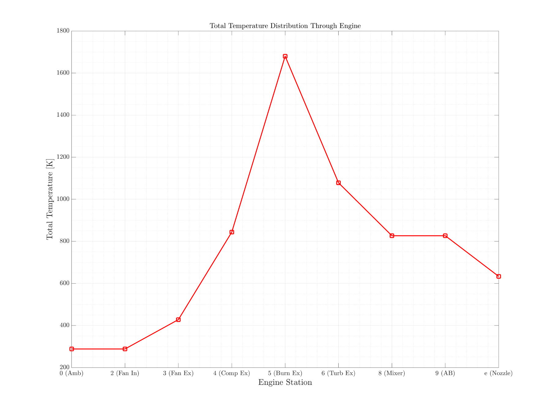
With the handout inputs, the model is within a few percent of the published thrust at military power and with afterburner. This agreement needs three qualifications:
- It is a comparison at one operating point in each mode.
- The ratings come from museum records and open literature. The model uses the handout’s ambient state (90.31 kPa, 288.15 K), and the report does not confirm that the ratings use the same state.
- The errors have opposite signs, high in dry mode and low with afterburner.
The report lists several possible causes for the remaining differences. They include the omitted turbine cooling and bleed flows, the idealized mixer, the frozen nozzle geometry and the property model. It did not test them separately, so I do not attribute the differences to any one of them.
The property model is a limitation in its own right. The specific-heat polynomials are fitted up to about 1200 K. The cycle reaches 1680 K at the turbine inlet and about 2035 K after the afterburner, so the model extrapolates at the hottest stations. The report estimates the resulting error as a few percent but does not quantify it.
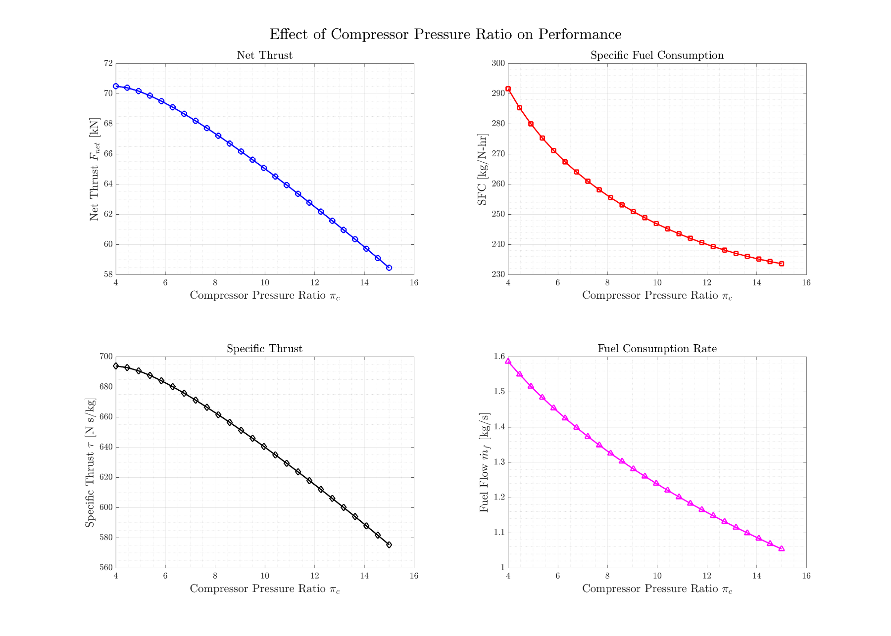
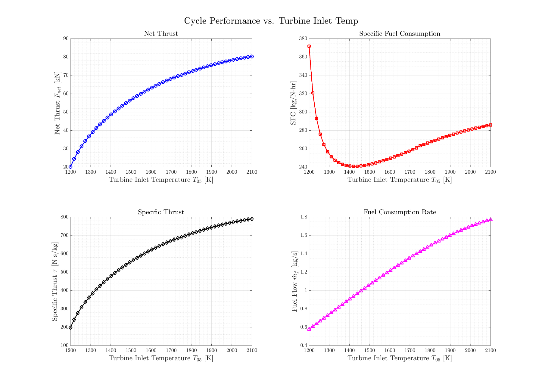
Parametric sweeps of turbine inlet temperature, compressor pressure ratio and component efficiency show the classic trade-offs within this model:
- Specific thrust increases with turbine inlet temperature, but SFC has a minimum near 1420 K in the sweep. The report links this minimum to the mixer momentum model, so it depends on that model.
- Over the swept range (\(\pi_c\) = 4–15), a higher compressor pressure ratio improves SFC but decreases specific thrust.
- Turbine efficiency has the strongest effect on thrust and SFC, and fan efficiency the weakest.
NotesCode provenance
The report describes MATLAB as the primary solver for the assessed results. It also documents Python scripts, which started as a translation of the MATLAB code and added alternative property models as auxiliary checks. Its appendix states that a consolidated Python script, derived from that translation, generated the figures and tables. The two statements are not fully consistent, so I describe the model as a MATLAB solver with a Python translation.