PIV Feasibility Study: Can Native Exhaust Aerosol Seed the Jet?
Course projectA course project in turbulent shear flows. Lubrication-oil-derived material in the P200-SX exhaust complicates the emissions measurements. I asked whether that native aerosol could instead seed particle image velocimetry (PIV) of the jet. On paper, it does not pass, so the study supports controlled external seeding.
WhyCould a measurement problem become a tracer?
The P200-SX has an open-loop lubrication system [22, 30]. Material derived from the lubrication oil reaches the exhaust, and this complicates the particle and emissions measurements. This project turned the problem around. Could that same particle population act as a native tracer for PIV of the jet?
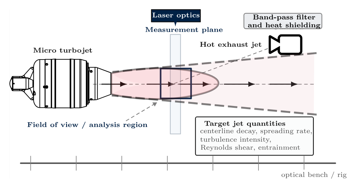
A velocity field would be useful. In a round jet, centerline decay, spreading, shear-layer structure, entrainment and the organization of turbulence are spatial properties of the plume. A point sensor gives local fluctuation levels. It cannot show how momentum and entrained air reorganize the plume in space [23, 24, 26, 37].
In a hot exhaust the need is sharper. The region that carries the transport physics also carries the experimental penalties: strong convection, density variation, tracer survival limits and difficult optical access.
The transport logic is compact. The velocity splits into a mean and a fluctuation. The turbulent kinetic energy summarizes the fluctuation level. The production term is the rate at which the mean flow feeds the turbulence:
In an axisymmetric jet, the Reynolds stresses and the mean gradients across the outer shear layer dominate production. A field measurement recovers the mean motion, the fluctuations and the gradients in one dataset.
The exit scales of the P200-SX are already demanding: \(D_j\approx67\) mm, \(U_e\approx490\) m s⁻¹ and \(Re_D\sim\mathcal{O}(10^5)\). The question was narrow. Can PIV work credibly in this plume, with the oil-derived particles as the only seed [22, 30]?
ScopeFour particle populations, kept separate
The word “aerosol” covers several different things here. I keep four of them apart:
- Native unstripped aerosol. This is what the study used. The SMPS sampled the exhaust with the catalytic stripper bypassed. It can hold soot, oil-derived droplets, condensate and other semivolatile material in unknown proportions. It is not a volatile-only distribution.
- Stripped (non-volatile) aerosol. A catalytic stripper removes most of the volatile material before the instrument. The non-volatile distributions on the nvPM page are of this type. This study did not use them.
- Inferred volatile fraction. A comparison of stripped and unstripped scans can give an operational estimate of the volatile part. This study made no such estimate.
- Artificial PIV seed. A controlled external tracer of known material and size, for example a refractory powder or an oil-droplet aerosol. The study recommends it as the benchmark. No seed was used.
The particle data come from earlier test campaigns at a downstream sampling point. They are not synchronized or co-located with any laser sheet. The data export also has no explicit dilution-ratio field.
HowChoosing a PIV modality
I judged each option by what it can realistically measure in this exhaust. The targets are centerline decay, jet spreading, outer-shear-layer structure, selected Reynolds stresses and the large motions that drive entrainment [5, 10, 23, 32].
| Modality | Components | Optical burden | Seeding burden | Best use in this exhaust |
|---|---|---|---|---|
| Planar 2C–2D | \(u, v\) in sheet | Low | Most forgiving | First campaign: mean decay, spread and shear-layer structure |
| Stereo 3C–2D | \(u, v, w\) in sheet | Moderate–high | Good image pairs in both views | Upgrade for entrainment and three-component transport |
| Tomographic 3C–3D | \(u, v, w\) in volume | High | Dense, uniform volume seeding | Only after tracer quality is established |
| Time-resolved planar | \(u, v\) in sheet | High | Long-record stability | Coherent structures and interface dynamics after a validated baseline |
| Time-resolved stereo | \(u, v, w\) in sheet | Very high | High-quality paired views over long records | Only when seeding and calibration are reliable |
Planar 2C–2D PIV is the defensible starting point. It recovers the most useful observables and puts the smallest demand on a tracer field of uncertain quality. Its main limit is the missing out-of-plane component [10, 27]. That matters only when the objective moves to entrainment paths or three-dimensional structure. Stereo, volumetric and time-resolved methods come later [3, 6, 24, 32, 36].
HowFive gates for a tracer
Hot-jet PIV usually fails at the tracer before it fails at the correlation algorithm. A usable tracer must pass five gates [1, 5, 27, 32]:
- It follows the resolved motion.
- It scatters enough light.
- It survives the thermal path to the imaging plane.
- It fills the light sheet densely and uniformly.
- It stays interpretable as one tracer class.
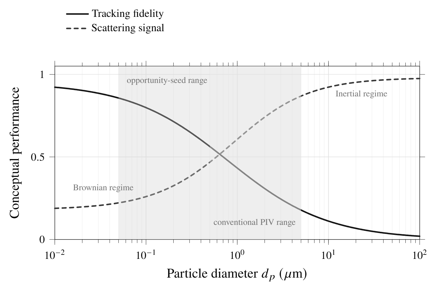
Gate 1, dynamic response. In the Stokes-drag limit:
Particle density \(\rho_p\), diameter \(d_p\), gas viscosity \(\mu\) and a characteristic flow timescale \(\tau_f\) [8, 27]. Low inertia is necessary but not sufficient.
Gate 2, scattering. The size parameter sets the regime. In the Rayleigh limit, the scattered intensity falls with the sixth power of the diameter:
Half the particle diameter means 1/64 of the signal [12, 27]. The plausible range for lubricant-derived particles here is roughly 50–500 nm. That is well below the low-micron size usually preferred in gas-phase PIV.
Gate 3, thermal survival. Refractory solids (alumina, titania, zirconia) tolerate high temperature. Their high density gives a longer relaxation time. Liquid tracers such as DEHS or glycol–water are bright at modest size. But in a hot flow they evaporate, change chemically and suffer thermophoretic loss [5, 27].
Gate 4, spatial adequacy. This gate is statistical. Correlation responds only to the particle images inside each interrogation window. Sparse, patchy or dim seeding broadens the peaks and biases the statistics [17, 36].
Gate 5, interpretive control. The signal can come from a mix of droplets, soot aggregates and condensate. Then neither the drag scale nor the optical scale belongs to one particle class [31, 33, 38].
| Material | Type | Typical \(d_p\) | \(\rho_p\) [kg m⁻³] | \(\tau_p\) at 1 µm | Survivable \(T\) | Scattering |
|---|---|---|---|---|---|---|
| Al₂O₃ | Solid | 0.3–5 µm | ∼3900 | ∼12 µs | High | Strong |
| TiO₂ | Solid | 0.2–3 µm | ∼4200 | ∼13 µs | High | Strong |
| ZrO₂ | Solid | 0.3–5 µm | ∼5600 | ∼17 µs | Very high | Strong |
| DEHS | Liquid | 0.5–3 µm | ∼910 | ∼2.8 µs | Low–moderate | Moderate |
| Glycol–water | Liquid | 0.5–5 µm | ∼1030 | ∼3.2 µs | Low–moderate | Moderate |
| Polystyrene | Solid | 0.2–2 µm | ∼1050 | ∼3.2 µs | Low | Moderate |
| Smoke | Mixed | < 0.5 µm | Variable | Very small | Variable | Weak |
| Lubricating oil (est.) | Liquid / condensate | 0.05–0.5 µm | ∼850–950 | ∼0.03–0.8 µs | Uncertain | Weak |
HowMeasurement limits
Different quantities fail at different points. Means converge first. Reynolds stresses need more samples and better peaks. Gradients, vorticity and entrainment metrics are the most fragile, because the estimator has already filtered the field they come from [23, 24, 36]:
\(G_I\) is the effective interrogation-window kernel. Window size, overlap, deformation and image weighting set it [26, 27].
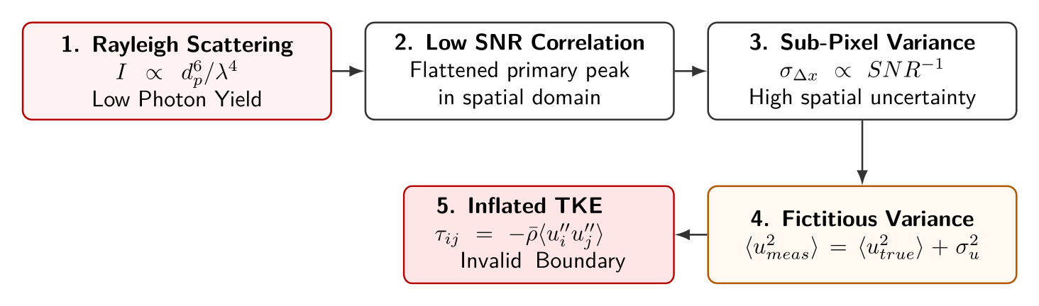
Uncorrelated measurement noise adds directly to the apparent fluctuation energy. Weak images therefore inflate the Reynolds stresses before they visibly distort the mean [16, 34, 36]:
At \(u'/U\approx0.15\) and \(U=490\) m s⁻¹, noise of \(\sigma_{n,u}=5\) m s⁻¹ barely changes the intensity. The same noise matters much more in the outer plume, where \(U\) drops and the signal weakens. This is how weak native seeding can produce false turbulent kinetic energy that varies in space.
The dynamic velocity range turns that hierarchy into a design problem. The particle-image displacement and the range that one setup can resolve are [1, 27]:
Magnification \(M_{\mathrm{opt}}\), local speed \(U\), pulse separation \(\Delta t\) and pixel pitch \(p\). No single \(\Delta t\) keeps both the 490 m s⁻¹ core and the slow entrained edge inside the preferred displacement band.
The first measurement window is therefore the early-development region, roughly \(x/D_j\approx2\text{–}6\). There, the shear layer is active and decay and spreading are emerging. The window also avoids the most hostile optical zone at the nozzle lip [15, 23, 24, 32].
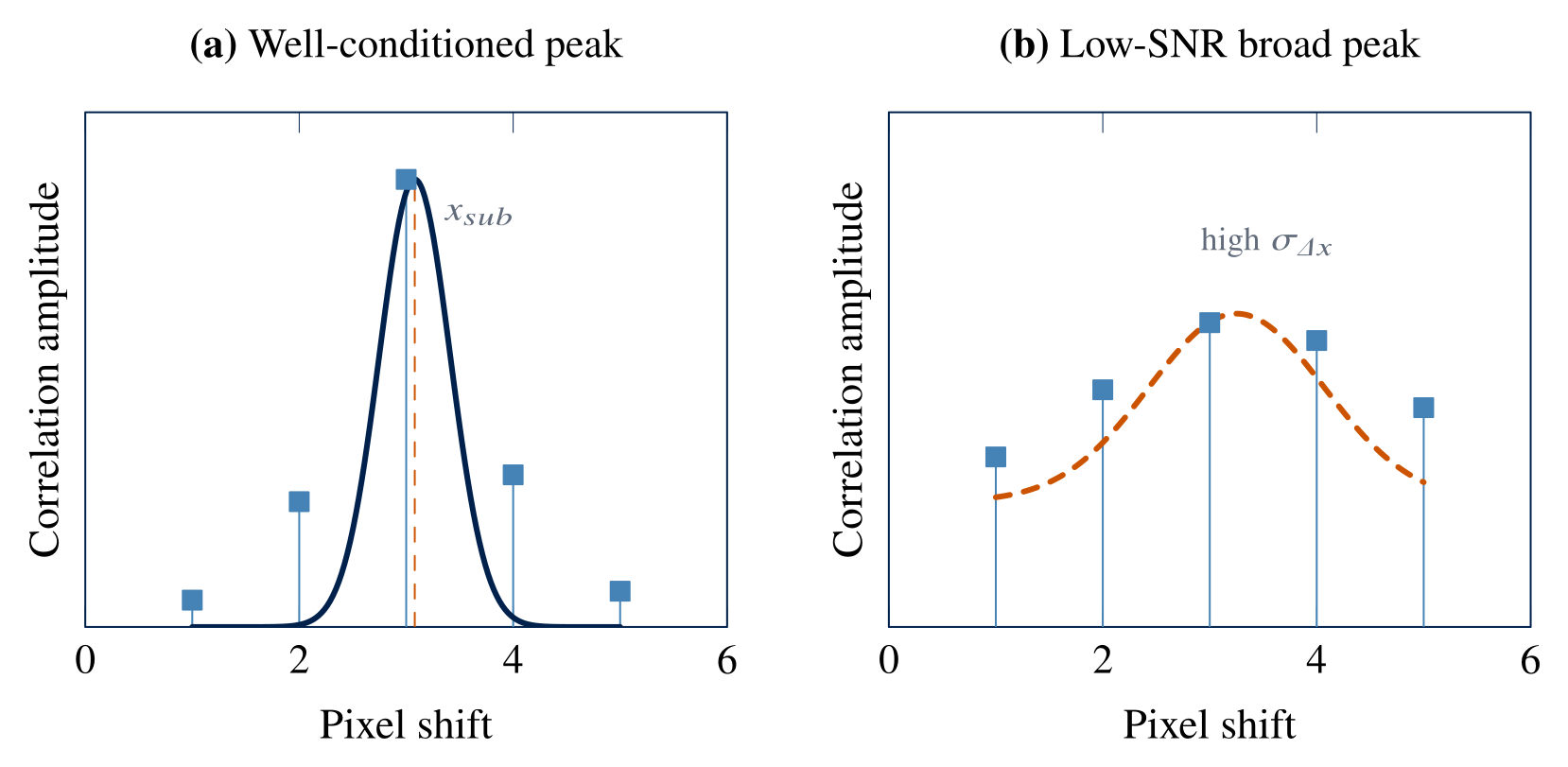
Correlation is a windowed similarity estimate. A three-point Gaussian fit refines the peak to sub-pixel precision. A normalized-median test then validates the vectors before any replacement, smoothing or differentiation [17, 27, 34, 35]:
The sub-pixel step only interpolates the peak that the image pair already made. When the peak is broad or noisy, the algebra still works, but the result loses physical credibility.
HowEngine context and the seeding hypothesis
| Quantity | Working design value |
|---|---|
| Nozzle diameter, \(D_j\) | 67 mm |
| Exit speed, \(U_e\) | ≈ 490 m s⁻¹ |
| Hot kinematic viscosity, \(\nu_h\) | (0.8–1.0) × 10⁻⁴ m² s⁻¹ |
| Reynolds number, \(Re_D=U_eD_j/\nu_h\) | \(\mathcal{O}(10^5)\) |
| Target image shift | 6–8 px |
| Estimated pulse separation | ≈ 0.8–1.3 µs |
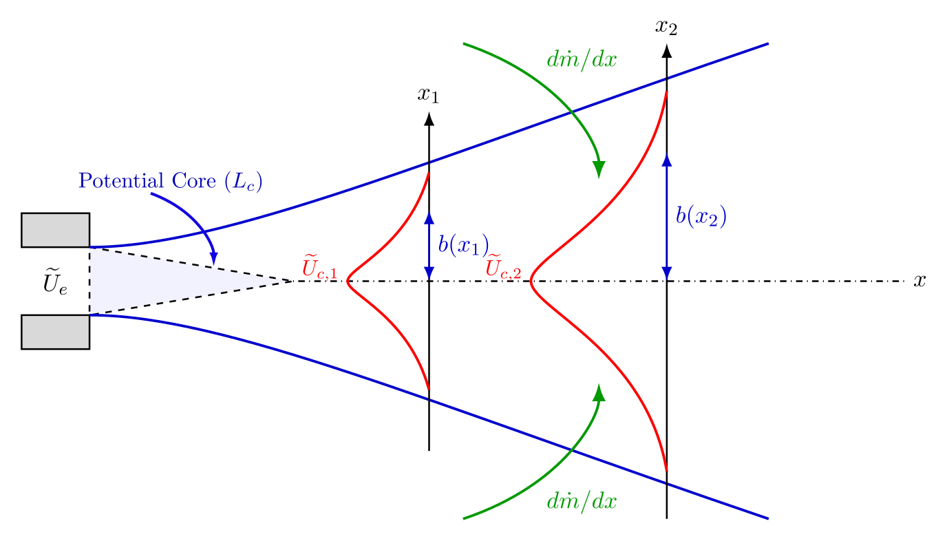
For a first-order plume analysis, the nozzle is a turbulent round-jet source. The exit momentum is approximately conserved, while the mass flow grows by entrainment [11, 19, 24, 37]:
Jet width \(b(x)\), centerline velocity \(U_c(x)\) and entrainment coefficient \(\alpha\). These are what PIV must recover to be useful. With the 6–8 px target shift, the displacement relation gives an inter-frame delay of about 0.8–1.3 µs. The report does not state the image scale behind this range, so it is a planning value only.
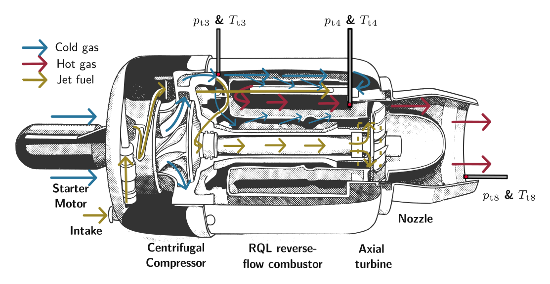
The hypothesis is narrow. The engine does not inject a controlled, monodisperse tracer. Downstream material can come from survival, cracking, reformation and condensation of the oil, and from mixing with soot or other semivolatile species [31, 33, 38].
A native tracer matters only if the material at the imaging plane passes all five gates. The particle data can test only part of that chain.
ResultsWhat the particle data show
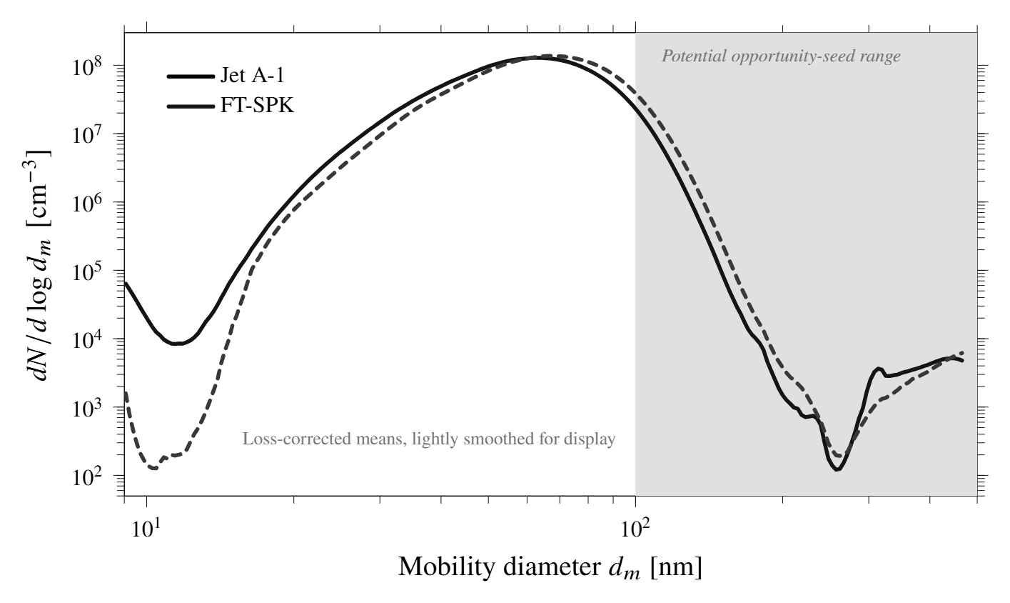
The data are three usable long-DMA SMPS scans per fuel at the matched 100% point, over 9.06–465.55 nm. They are loss-corrected and given as \(\mathrm{d}N/\mathrm{d}\log d_m\). That is mobility-diameter space, which differs from optical diameter [13, 14, 21, 30].
| Jet A-1 | FT-SPK | |
|---|---|---|
| Mode (unstripped) | 65.52 nm | 67.93 nm |
| Total number concentration | 4.12 × 10⁷ cm⁻³ | 4.27 × 10⁷ cm⁻³ |
| 100–500 nm tail | 9.36 × 10⁵ cm⁻³ | 1.76 × 10⁶ cm⁻³ (1.88×) |
| Fraction below 100 nm | 97.73% | 95.88% |
| 200–465.55 nm sub-band | 9.01 × 10² cm⁻³ | 7.73 × 10² cm⁻³ |
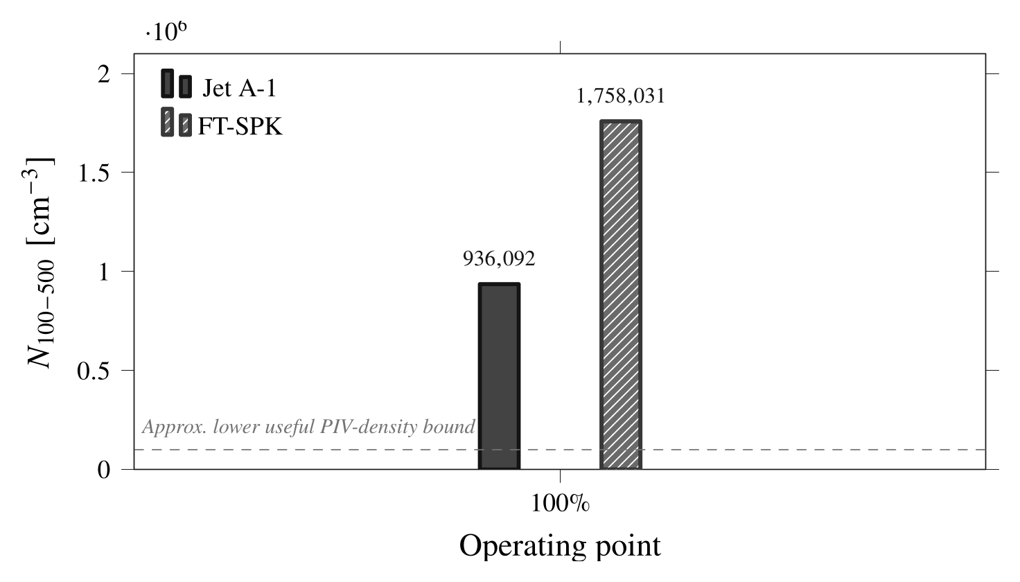
These concentrations give a first-pass image-density estimate. Take a volumetric concentration \(N_v\) in a light sheet of thickness \(\Delta z_0\). Use a representative 32 × 32 px window at 0.1 mm px⁻¹:
With \(\Delta z_0=1\) mm, the full 100–500 nm tail gives \(N_{IW}\approx9.6\times10^{3}\) (Jet A-1) and \(1.8\times10^{4}\) (FT-SPK). That is far above the Keane–Adrian guideline of 10–15 images per window [17]. The more optically promising 200–465.55 nm sub-band gives only \(N_{IW}\approx9.2\) and \(7.9\). These are upper bounds. They count every particle in the band as visible, and the concentrations apply at the sampling point.
Four limits stop this from being a positive result:
- Mobility diameter is not the compact optical diameter for fractal soot [7, 13, 18, 21].
- With the stripper bypassed, soot, oil-derived droplets and semivolatile material are counted together [31, 33, 38].
- The SMPS counts what reached the instrument, which can differ from what crosses a laser sheet.
- No data show that the optically useful fraction survives the path through the combustor, turbine and nozzle.
ResultsGate-by-gate verdict
A worked example: a 200 nm droplet-like particle, with Sutherland’s law for air at 800 K.
\(\mu_0=1.716\times10^{-5}\) Pa s, \(T_0=273.15\) K, \(S=110.4\) K, \(\tau_f=D_j/U_e=0.067/490\approx1.37\times10^{-4}\) s. The density of 850 kg m⁻³ is an assumed, droplet-like value.
| Proxy \(d_p\) | \(\tau_p\) [s] | \(St\) | \(x\) at 532 nm | Regime |
|---|---|---|---|---|
| 100 nm | 1.30 × 10⁻⁸ | 9.52 × 10⁻⁵ | 0.59 | Mie / transitional |
| 200 nm | 5.21 × 10⁻⁸ | 3.81 × 10⁻⁴ | 1.18 | Mie / transitional |
| 300 nm | 1.17 × 10⁻⁷ | 8.57 × 10⁻⁴ | 1.77 | Mie / transitional |
| 500 nm | 3.26 × 10⁻⁷ | 2.38 × 10⁻³ | 2.95 | Mie / transitional |
| Gate | Evidence | Verdict |
|---|---|---|
| Tracking fidelity | \(St=9.5\times10^{-5}\) to \(2.4\times10^{-3}\) over 100–500 nm, if the particles are droplet-like | Favorable |
| Scattering at 532 nm | \(x=0.59\text{–}2.95\), but only 2.27% (Jet A-1) and 4.12% (FT-SPK) of particles are in 100–500 nm | Marginal |
| Thermal survival | A population reaches the SMPS. Survival of the optically useful fraction to the sheet is unmeasured. | Unknown |
| Spatial adequacy | Upper-bound \(N_{IW}\approx9.6\times10^3\) and \(1.8\times10^4\). The 200–465 nm sub-band gives only ≈ 9.2 and 7.9. | Unknown / unfavorable |
| Interpretive control | The stripper bypass mixes soot, oil-derived and semivolatile material. \(d_m\) is not the optical diameter for aggregates. | Marginal |
The result is negative for quantitative PIV. The particles track well, and the 100–500 nm tail is not zero. The native aerosol might therefore show plume structure qualitatively. But the optically useful particles are a minority tail. Their survival and spatial uniformity are unknown, and the SMPS cannot separate soot from oil-derived material.
ResultsWhat the study supports
The study supports controlled external seeding for any quantitative PIV of this jet. The report described a gated test path to check this, shown below as a planning diagram. None of these phases was carried out.
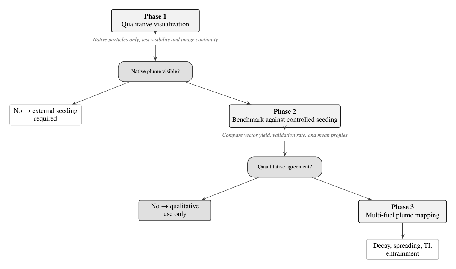
- Visibility check: native particles only, one sheet and one view, in the \(x/D_j\approx2\text{–}6\) window. The gate is repeatable plume structure. Isolated speckles do not count.
- Benchmark: the same optics, field of view, pulse separation and processing, with a controlled external seed. Success means an acceptable vector yield and validation rate, and mean profiles that agree within the expected uncertainty.
- Fuel comparison: planar PIV mapping of the plume for each fuel, with stereo only after the tracer is trusted.
RelevanceWhy the jet matters beyond the nozzle
Downstream of the nozzle, the exhaust is an entraining free jet. Species transport there follows momentum, mass and entrainment. The well-stirred and plug-flow idealizations used inside the combustor do not apply [22, 25]. The jet growth and centerline decay set the dilution history and the time available for chemistry, oxidation or condensation:
The last pair is a one-dimensional plume reactor that could extend a combustor reactor network. A measured jet growth would fix \(E(x)\), and a measured decay would fix \(\tau_c\). FANS and LES plume models need the same transport closure before their species, soot or ice predictions can be trusted [2, 3, 4, 20, 28].
This is the wider reason for the project. The jet spreads, its shear layers entrain air, and the mixing sets how fast the exhaust dilutes and cools. This transport is coupled to the fuel-dependent particle populations that the program measures.
Controlled-seed PIV plus matched native-aerosol measurements could constrain hypotheses about particle transport, evolution and activation. Matched means the same operating point, with known sampling positions and dilution, and both unstripped and stripped scans.
Size distribution and velocity alone do not determine cloud-condensation-nucleus activity or contrail ice. That also needs temperature, humidity, particle composition and hygroscopicity, and activation measurements or a suitably constrained model.
References
- [1]R. J. Adrian and J. Westerweel, Particle Image Velocimetry, Cambridge Aerospace Series, vol. 30. Cambridge University Press, 2011.
- [2]C. M. Arndt, M. Severin, C. Dem, M. Stöhr, A. M. Steinberg and W. Meier, “Experimental analysis of thermo-acoustic instabilities in a generic gas turbine combustor by phase-correlated PIV, chemiluminescence, and laser Raman scattering measurements,” Experiments in Fluids, 56(4), 69, 2015.
- [3]M. A. Brend, P. A. Denman and J. F. Carrotte, “Volumetric PIV measurement for capturing the port flow characteristics within annular gas turbine combustors,” Experiments in Fluids, 61(4), 106, 2020.
- [4]C. Chelem Mayigue, I. R. Jahncke, T. M. Taddesse, C. P. T. Groth, A. Roy, R. Sawanni, Y. T. Rajan, S. Chaudhuri and Ö. L. Gülder, “Contrail formation simulation via FANS-based turbulence modelling combined with two-equation soot/ice particle transport modelling,” AIAA SciTech Forum, AIAA Paper 2025-0600, Orlando, FL, 2025.
- [5]F. Chen and H. Liu, “Particle image velocimetry for combustion measurements: applications and developments,” Chinese Journal of Aeronautics, 31(7), 1407–1427, 2018.
- [6]B. Coriton and J. H. Frank, “Experimental study of vorticity-strain rate interaction in turbulent partially premixed jet flames using tomographic particle image velocimetry,” Physics of Fluids, 28(2), 025109, 2016.
- [7]L. Durdina et al., “Reduction of nonvolatile particulate matter emissions of a large turbofan engine burning a SAF blend,” Environmental Science & Technology, 55, 14576–14585, 2021.
- [8]C. Fang et al., “Tracking characteristics of tracer particles for PIV measurements in supersonic flows,” Chinese Journal of Aeronautics, 2017.
- [9]A. Fushimi et al., “Identification of jet lubrication oil as a major component of aircraft exhaust nanoparticles,” Atmospheric Chemistry and Physics, 19, 6389–6399, 2019. Note: the authors have withdrawn this paper.
- [10]B. Ganapathisubramani, K. Lakshminarasimhan and N. T. Clemens, “Investigation of three-dimensional structure of fine scales in a turbulent jet by using cinematographic stereoscopic particle image velocimetry,” Journal of Fluid Mechanics, 598, 141–175, 2008.
- [11]D. Han and M. G. Mungal, “Direct measurement of entrainment in reacting/non-reacting jets in coflow using PIV,” Combustion and Flame, 126(1–2), 1438–1442, 2001.
- [12]M. F. Hantke et al., “Rayleigh-scattering microscopy for tracking and sizing nanoparticles in focused aerosol beams,” IUCrJ, 2018.
- [13]W. C. Hinds, “Physical and chemical processes in aerosol systems,” in Aerosol Measurement: Principles, Techniques, and Applications, 3rd ed., pp. 31–40. Wiley, 2011.
- [14]W. John, “Size distribution characteristics of aerosols,” in Aerosol Measurement: Principles, Techniques, and Applications, 3rd ed., pp. 41–54. Wiley, 2011.
- [15]P. Karra, T. Rogers and P. Lappas, “Air entrainment in gaseous fuel jets using particle image velocimetry and high speed schlieren photography in a constant volume chamber,” SAE Technical Paper 2015-01-0938, 2015.
- [16]S. M. Kay, Intuitive Probability and Random Processes using MATLAB. Springer, 2006.
- [17]R. D. Keane and R. J. Adrian, “Theory of cross-correlation analysis of PIV images,” Applied Scientific Research, 49, 191–215, 1992.
- [18]G. A. Kelesidis et al., “Toward elimination of soot emissions from jet fuel combustion,” ACS, 2023.
- [19]G. Kewalramani, B. Ji, Y. Dossmann, S. Becker, M. Gradeck and N. Rimbert, “A simple analytical model for turbulent kinetic energy dissipation for self-similar round turbulent jets,” Journal of Fluid Mechanics, 983, A44, 2024.
- [20]P. Koob et al., “Large eddy simulation of soot formation in a real aero-engine combustor using tabulated chemistry,” Journal of Engineering for Gas Turbines and Power, 146(1), 2024.
- [21]P. Kulkarni, P. A. Baron and K. Willeke (eds.), Aerosol Measurement: Principles, Techniques, and Applications, 3rd ed. Wiley, 2011.
- [22]D. Lieder, S. Sharma, P. Kirchen, S. Rogak and J. Goeing, “Development of a validated chemical reactor network model for non-CO₂ emissions in RQL aircraft combustors,” Proc. ASME Turbo Expo 2026, GT2026-177253, Milan, 2026.
- [23]J. Mi, P. Kalt, G. J. Nathan and C. Y. Wong, “PIV measurements of a turbulent jet issuing from a round sharp-edged orifice plate,” Experiments in Fluids, 42(4), 625–637, 2007.
- [24]D. Mistry, J. Philip, J. R. Dawson and I. Marusic, “Entrainment at multi-scales across the turbulent/non-turbulent interface in an axisymmetric jet,” Journal of Fluid Mechanics, 802, 2016.
- [25]A. Mukhopadhyay and S. Sen, Fundamentals of Combustion Engineering. CRC Press, 2019.
- [26]S. B. Pope, Turbulent Flows. Cambridge University Press, 2000.
- [27]M. Raffel, C. E. Willert, F. Scarano, C. J. Kähler, S. T. Wereley and J. Kompenhans, Particle Image Velocimetry: A Practical Guide, 3rd ed. Springer, 2018.
- [28]A. Savitskii, A. Lobasov, D. Sharaborin and V. Dulin, “Testing basic gradient turbulent transport models for swirl burners using PIV and PLIF,” Fluids, 6(11), 383, 2021.
- [29]R. Schiestel, Modeling and Simulation of Turbulent Flows. ISTE and Wiley, 2008.
- [30]S. Sharma, D. Lieder, S. Saini, A. Kumar, P. Kirchen, J. Goeing and S. Rogak, “A micro-turbojet test rig to analyze the impact of jet fuels on emissions and performance,” Proc. CSME-CFDSC-CSR 2026, accepted.
- [31]M. T. Timko et al., “Characterization of lubrication oil emissions from aircraft engines,” Environmental Science & Technology, 2010.
- [32]B. H. Timmerman, A. J. Skeen, P. J. Bryanston-Cross and M. J. Graves, “Large-scale time-resolved digital particle image velocimetry (TR-DPIV) for measurement of high subsonic hot coaxial jet exhaust of a gas turbine engine,” Measurement Science and Technology, 20(7), 074002, 2009.
- [33]M. Ungeheuer et al., “Nucleation of jet engine oil vapours is a large source of aviation ultrafine particles,” Communications Earth & Environment, 2022.
- [34]J. Westerweel, “Fundamentals of digital particle image velocimetry,” Measurement Science and Technology, 8(12), 1997.
- [35]J. Westerweel and F. Scarano, “Universal outlier detection for PIV data,” Experiments in Fluids, 39, 1096–1100, 2005.
- [36]B. Wieneke, “PIV uncertainty quantification from correlation statistics,” Measurement Science and Technology, 26, 074002, 2015.
- [37]I. Wygnanski and H. Fiedler, “Some measurements in the self-preserving jet,” Journal of Fluid Mechanics, 38(3), 577–612, 1969.
- [38]Z. Yu et al., “Identification of lubrication oil in the particulate matter emissions from commercial aircraft,” Environmental Science & Technology, 2012.