WhatWhy non-volatile particles

Non-volatile particulate matter (nvPM) is essentially soot. It is now regulated for aircraft engines, and soot particles can act as nuclei for contrail ice. Three quantities matter: how many particles an engine emits, how large they are, and how both respond to fuel composition. Low-aromatic sustainable fuels are expected to cut soot. But full-scale data cannot easily separate fuel effects from engine and operating effects [1, 3].

The micro-turbojet makes these measurements controllable and repeatable. This work asks whether its particles are representative, and how much the result depends on how the sample is taken.

HowMeasuring particles a few nanometers across

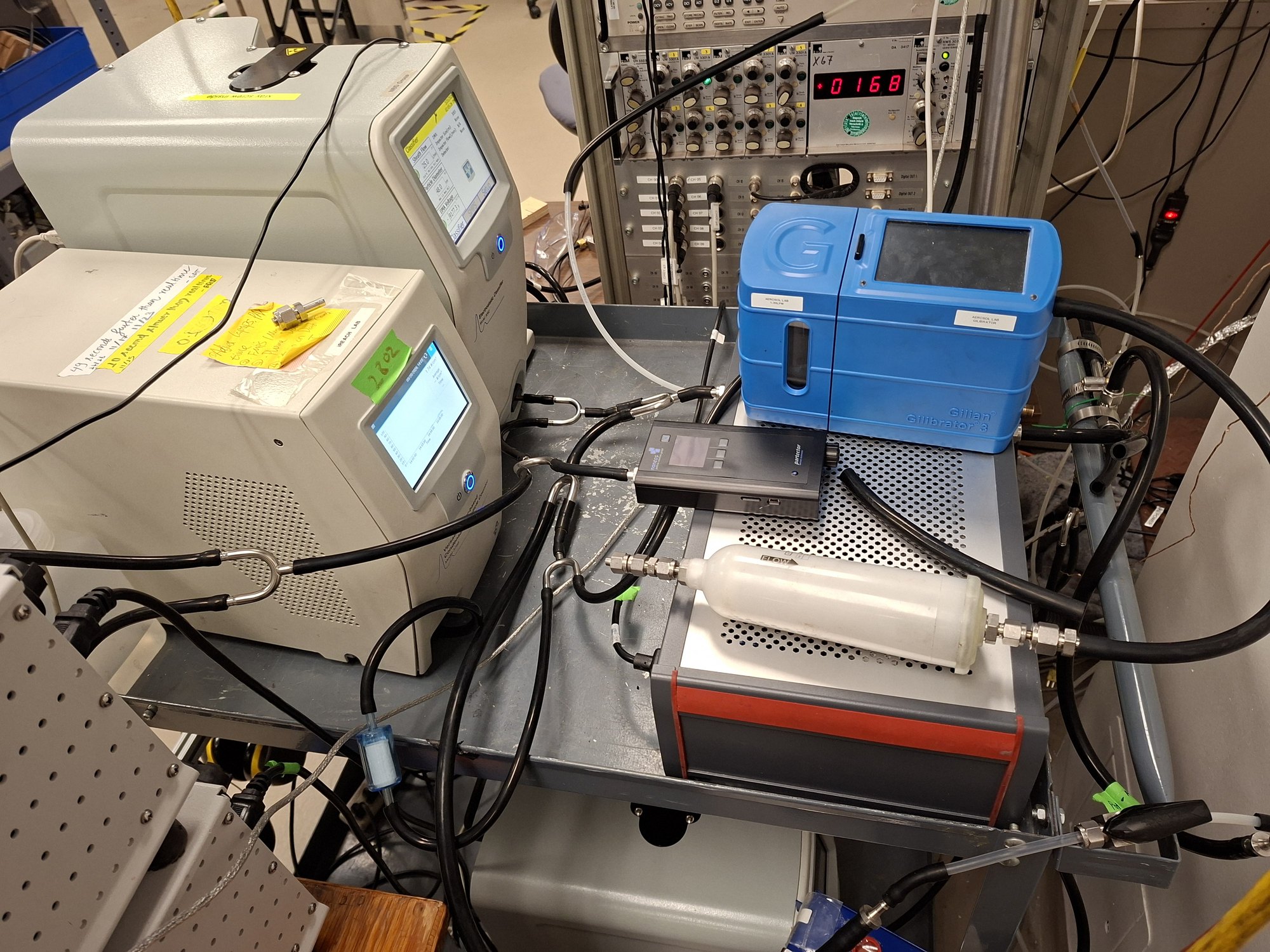
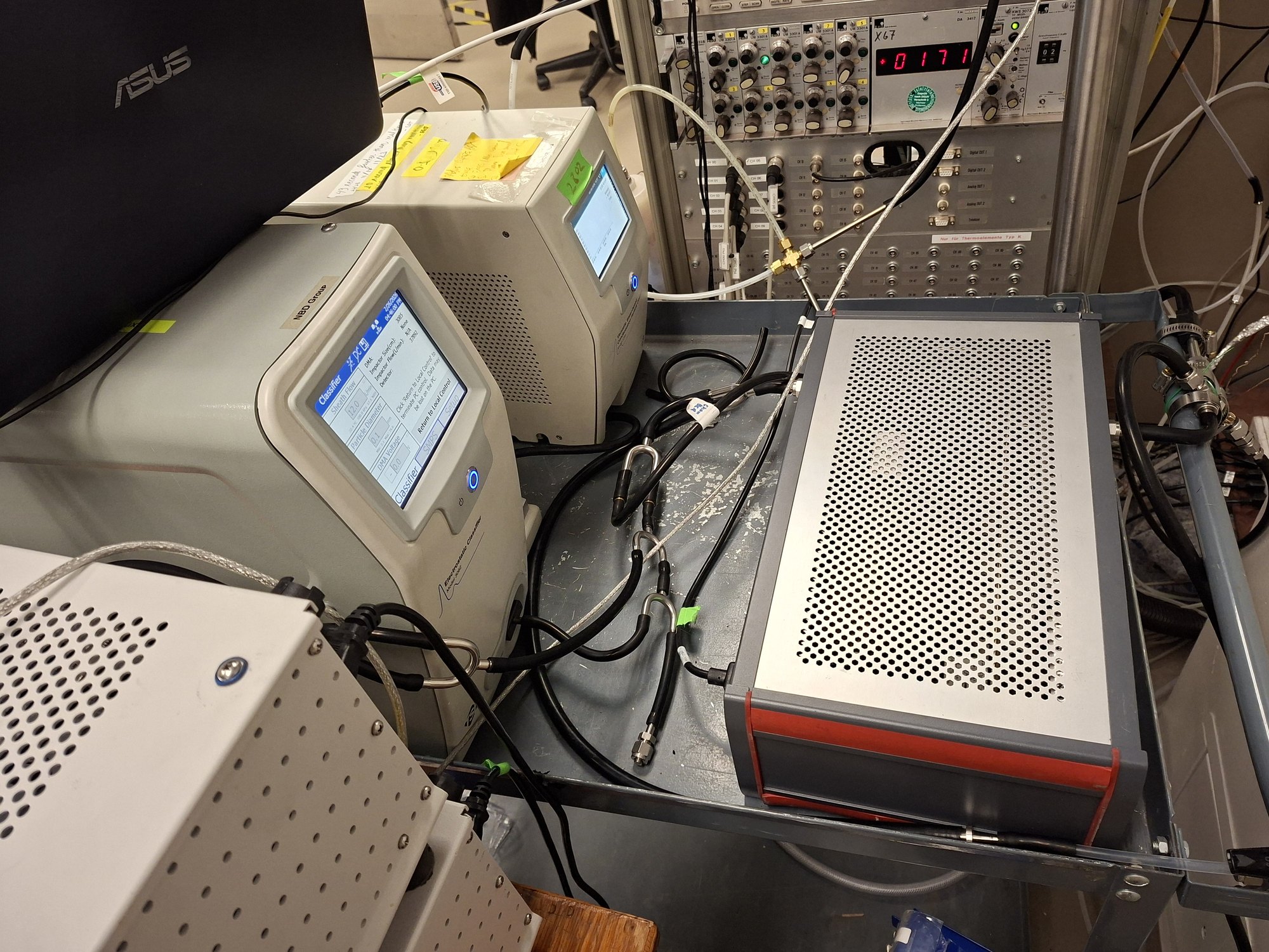
The exhaust goes through an ejector diluter into the diluted line. A catalytic stripper removes volatile material, so only non-volatile particles reach the scanning mobility particle sizer (SMPS). In the SMPS, a nano-DMA classifies the particles by electrical mobility, and a water-based condensation particle counter counts them. Each scan takes 120 s with a 30 s purge, at 1.5 L/min sample flow and 12 L/min sheath flow [2].

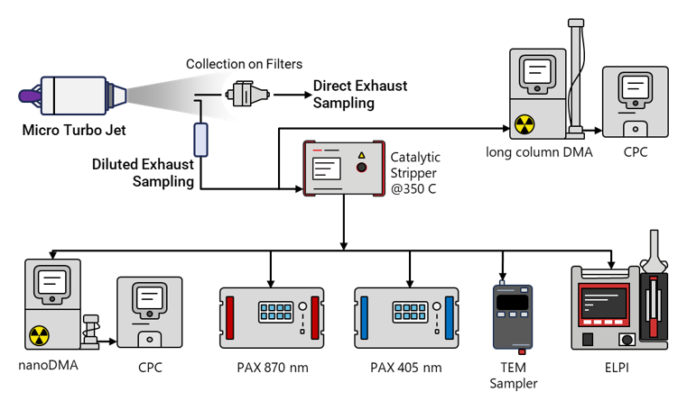
The Method view in the gallery at the top is a schematic of the full particle train. Besides the nano-SMPS, it shows:

• a long-column DMA and CPC on a branch ahead of the stripper
• absorption and scattering photometers at 405 and 870 nm
• an electrical low-pressure impactor
• a sampler that collects particles on TEM grids for morphology.

The results on this page come only from the nano-SMPS. They do not include optical or morphology data.

HowCorrecting for what the sampling line removes

At these sizes, the sampling system itself is a large part of the measurement. Brownian diffusion to the tube walls, settling, turbulent deposition and the stripper all remove particles before the counter sees them. The fraction they remove depends on size.

I built the correction bin by bin. I divide each measured mobility-diameter bin by the total penetration of the train. I do not fit an assumed lognormal engine-exit distribution. The comparison between fuels therefore uses the measured shape itself [6].

I modeled the diluted line as six straight circular segments:

• probe to ejector
• the ejector block, as one equivalent section
• the main transfer line
• the branch
• the run to the stripper
• the run from the stripper to the SMPS.

The flow rate and diameter of each segment give its velocity and Reynolds number. Only the ejector block (Re ≈ 11,200) is treated as turbulent. The transfer sections (Re ≈ 1,900–2,200) are in the transition range, and the code forces them to the laminar branch. That is an implementation choice [6]. Within a segment, the loss mechanisms multiply:

Particle mobility enters through the Cunningham slip correction. This correction sets both the Brownian diffusion coefficient and the Stokes number:

Diffusion dominates for the smallest particles. In the laminar segments, it follows the Gormley–Kennedy solution in the deposition parameter \(\mu_{GK}=D_BL/Q\). In the turbulent segment, it follows a Sherwood-number correlation:

Settling and turbulent inertial deposition matter only for the larger sizes, but I keep them for completeness. The settling velocity is \(V_{ts}=\rho_pD_p^2gC_c/18\mu\). In the turbulent segment, the deposition velocity adds a loss that depends on the Stokes number:

In the catalytic stripper, diffusion and thermophoresis remove the smallest particles. Its penetration uses the manufacturer’s empirical fit, with the diameter in nanometers:

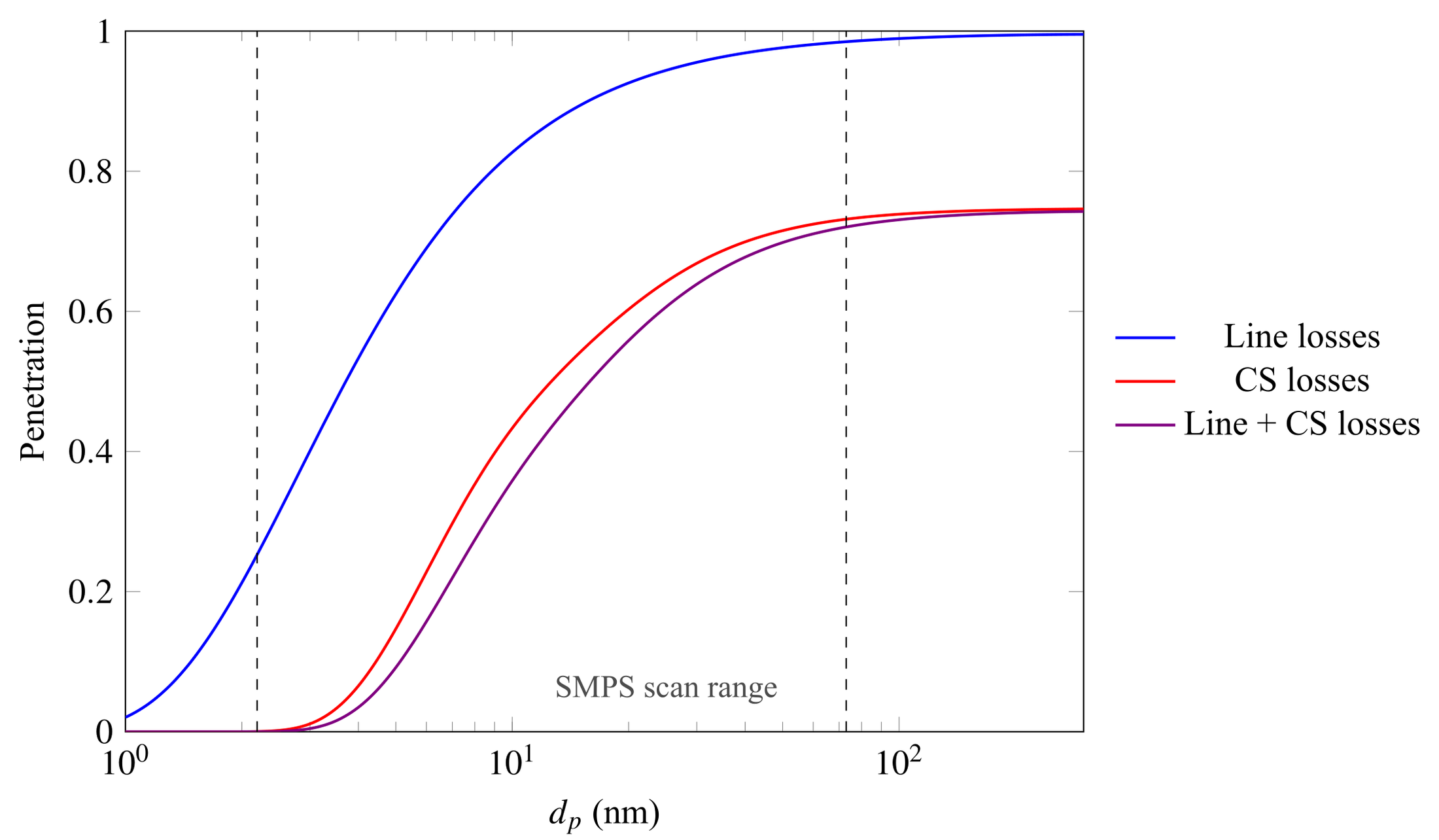
The stripper sets the shape of the correction. The lines alone pass more than 80% of particles above about 10 nm. But the combined train passes less than 40% at 10 nm and almost nothing near 3 nm. That is why the smallest bins carry the largest correction.

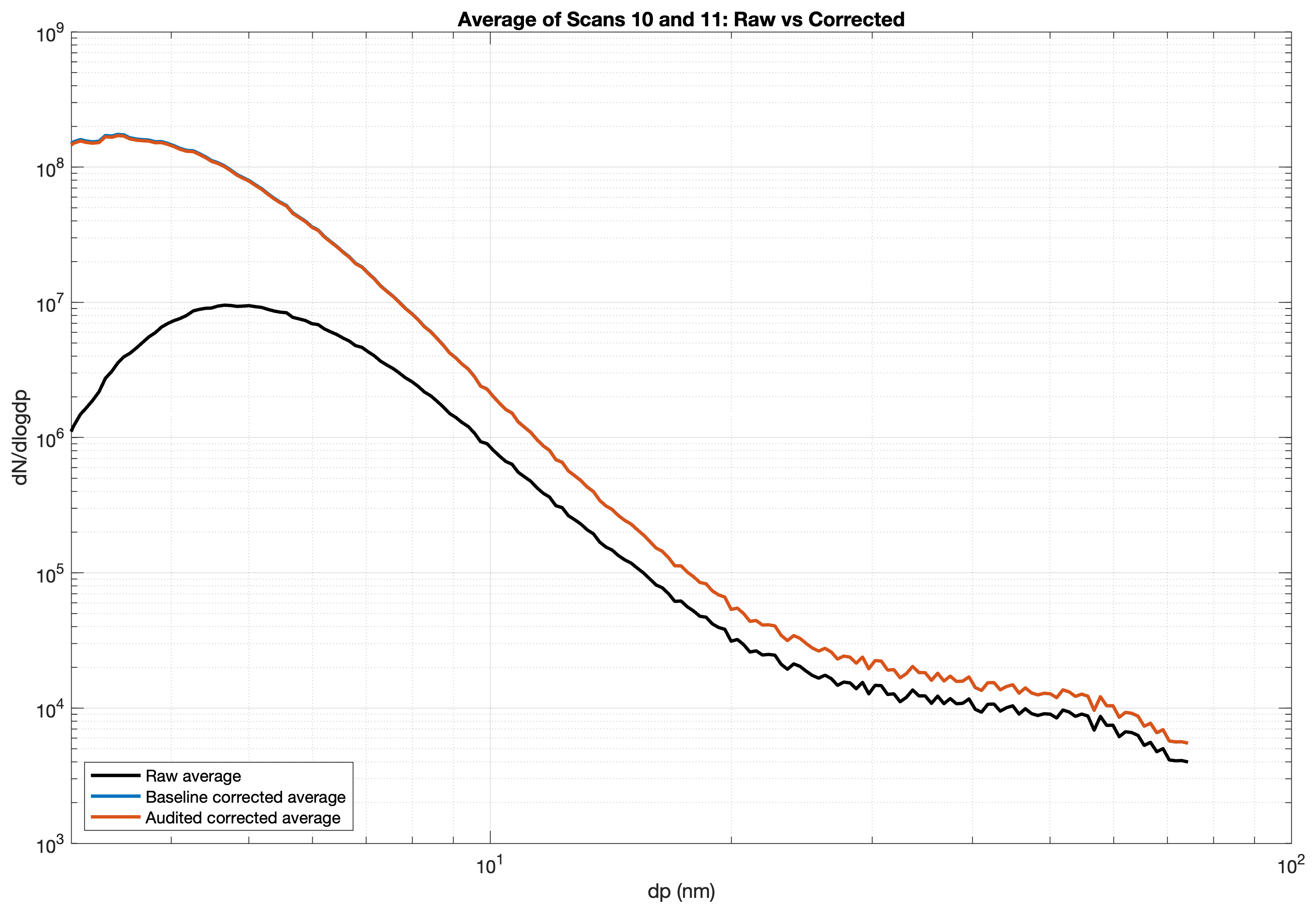
The number size distribution is the measured quantity. Mass is derived from it with two assumptions: spherical-equivalent particles, and a constant effective density of 1 g cm⁻³ (the ICAO convention). This is an equivalent-density approximation [3, 6].

Number and mass then go on the same carbon-balance basis as the gas emission indices:

ResultsUltrafine soot, similar in shape to a turbofan at idle

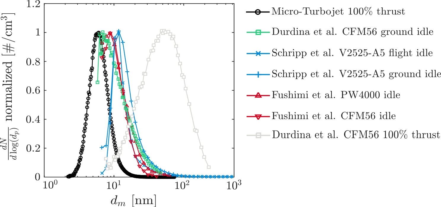
The Result view at the top compares the micro-turbojet with published turbofan data. Every curve is scaled to a maximum of 1, so it compares shape and position only. The turbofan data are CFM56 at ground idle and 100% thrust [4] and V2500-family engines at flight and ground idle [5]. The PW4000 and CFM56 idle curves come from Fushimi et al. Note: Fushimi et al. have withdrawn their paper. Their PW4000 and CFM56 idle curves are shown for completeness and should not be relied on.

In the first campaign, reported at CSME, the distribution at maximum thrust was mono-modal [1]. Three sizes describe it, and they are not the same quantity:

• the mode (the most frequent size): 7.84 nm
• the geometric mean diameter: 8.6 nm
• the geometric standard deviation: 1.44.

Durdina et al. report a mean diameter of about 8 nm for a CFM56-7B at ground idle with Jet A-1, with a wider distribution (GSD of about 2) [1, 4]. The micro-turbojet at maximum power therefore produces particles of a similar size to a large engine near idle. This matches the combustor-inlet comparison, but it is one engine and one operating point on each side.

The two curves also differ in method. Durdina et al. corrected their data for sampling-line losses. The CSME paper does not describe a loss correction for this first micro-turbojet distribution [1, 4].

The later loss-corrected emission-index distributions are a different quantity. Their number maximum is at 3.8, 3.9 and 4.3 nm for 50, 70 and 100% thrust. These sizes are inside the range where the loss correction is largest [2, 6].

ResultsFT-SPK: less soot mass, and an uncertain number change

Back-to-back at maximum thrust in the GPPS campaign, FT-SPK lowered the unit-density soot mass emission index by 72%. The number emission index rose by 38% [3]. These two results do not have the same reliability.

The number increase comes only from the smallest bins, where the scans scatter most and the loss correction is largest. Because those bins hold the most particles, they control the total number. Across almost the whole size range, the measured FT-SPK distribution is lower than Jet A-1 [3].

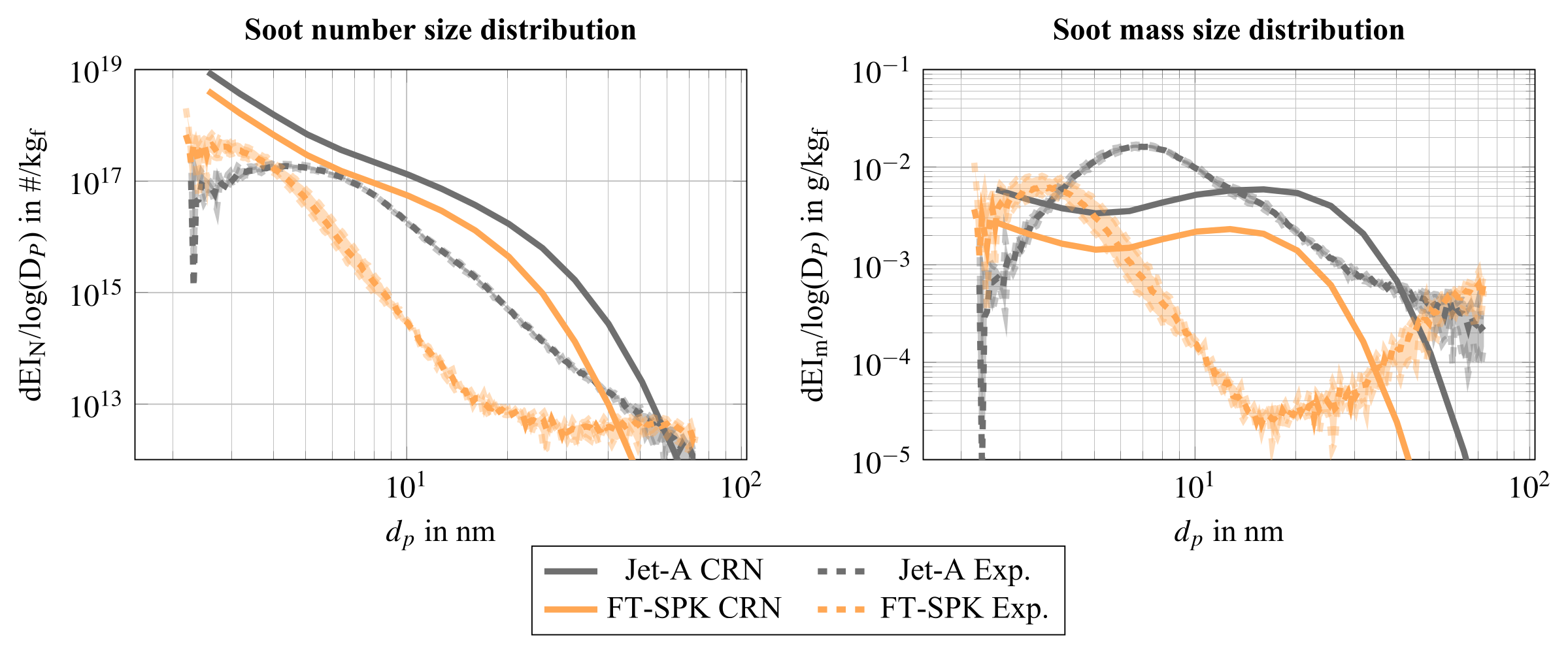
The measurements and the model both show the distribution moving to smaller diameters. The measured Jet A-1 number maximum is at about 4 nm. For FT-SPK, the slope inverts at about 3 nm, which indicates a maximum there [3].

The mass result has its own limit. Any constant density multiplies both fuels by the same factor, so it cancels in the ratio. The 72% reduction at 1, 1.5 and 1.86 g cm⁻³ therefore follows from the arithmetic [6].

A size-dependent effective density gives 71% [6]. That case applies the same density relation to both fuels. None of these cases measures particle morphology or a fuel-dependent density.

References

1. [1]S. Sharma, D. Lieder, S. Saini, A. Kumar, P. Kirchen, J. Goeing and S. Rogak, “A micro-turbojet test rig to analyze the impact of jet fuels on emissions and performance,” Proc. CSME International Congress / 33rd Annual Conf. CFD Society of Canada, Vancouver, May 2026, Paper 361.
2. [2]S. Sharma, D. Lieder, N. Sapkota, H. Lintusaari, A. Kumar, P. Kirchen, J. Goeing and S. Rogak, “Experimental and model characterization of jet fuel emissions in a micro-turbojet engine,” Combustion Institute – Canadian Section Spring Technical Meeting, Concordia University, May 2026.
3. [3]D. Lieder, S. Sharma, H. Lintusaari, N. Sapkota, A. Kumar, P. Kirchen, J. Friedrichs, S. Rogak and J. Goeing, “Measurement and prediction of particle emissions from a micro turbojet using conventional and alternative jet fuel,” Proc. GPPS Montreal26, GPPS-TC-2026-102, 2026, doi:10.33737/gpps26-tc-102. © the authors, CC BY-NC-ND 4.0.
4. [4]L. Durdina et al., “Reduction of nonvolatile particulate matter emissions of a commercial turbofan engine at the ground level from the use of a sustainable aviation fuel blend,” Environmental Science & Technology, 55, 14576–14585, 2021. (Source of the CFM56-7B comparison data.)
5. [5]T. Schripp et al., “Aircraft engine particulate matter emissions from sustainable aviation fuels: results from ground-based measurements during the NASA/DLR campaign ECLIF2/ND-MAX,” Fuel, 325, 124764, 2022. (Source of the V2500-family comparison data.)
6. [6]D. Lieder, S. Sharma, H. Lintusaari, N. Sapkota, A. Kumar, P. Kirchen, J. Friedrichs, S. Rogak and J. Goeing, “Supplementary information: Measurement and prediction of particle emissions from a micro turbojet using conventional and alternative jet fuel,” GPPS-TC-2026-102, 2026. (Loss-correction method, Eqs. 1–29 and Fig. 1.)