A Physics-Based Transient Micro-Turbojet Model
Graduate research · side projectI built a physics-based transient model of the P200-SX core with a P220 nozzle, in MATLAB and Simulink. It is built from component physics. Driven by the measured fuel flow, it predicts speed, thrust and several sensor readings. It also gives an estimate of the air mass flow, which the rig does not measure. That estimate is model-dependent and has no direct validation.
WhatWhy build a model
To report a global equivalence ratio for the combustor, I need the air mass flow into the engine. The rig measures fuel flow, spool speed, thrust and a few pressures and temperatures, but not air mass flow. Earlier estimates from nozzle-exit relations did not hold up. A dynamic engine model that reproduces the measured channels gives a model-based estimate of the missing flow.
The quantity the model was built to estimate. The rig does not measure \(\dot m_a\), so any value for it comes from the model.
Published micro-turbojet models usually do four things [1]:
- They scale generic component maps to a design point.
- They use constant gas properties.
- They compare model gas temperatures directly with thermocouple readings.
- They calibrate and assess on the same data.
I built this model to avoid all four.
HowArchitecture
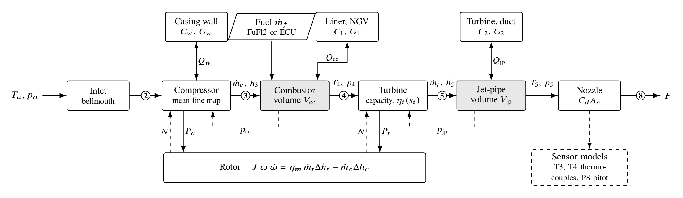
The engine is a chain of algebraic component models, joined by two gas volumes: the combustor (\(V_{cc}=7.35\times10^{-4}\) m³, from CAD) and the jet pipe (\(V_{jp}=3.20\times10^{-4}\) m³). The compressor, turbine and nozzle flows follow from the volume pressures and the shaft speed. As a result, the solver does not iterate a mass balance inside a time step. The plant has ten states [1]:
- the shaft speed
- the mass, internal energy and burnt-fuel mass in each volume
- three wall temperatures.
Mass and energy balance for each volume (\(\delta_{cc}=1\) in the combustor only) and for the rotor, with \(J=1.15\times10^{-4}\) kg m², \(\eta_m=0.98\) and an assumed \(\eta_b=0.935\). Temperature follows from \(U=m[h(T,f)-R(f)T]\) and pressure from \(p=mRT/V\), with NASA-polynomial properties for air and lean products.
HowComponent physics instead of scaled maps
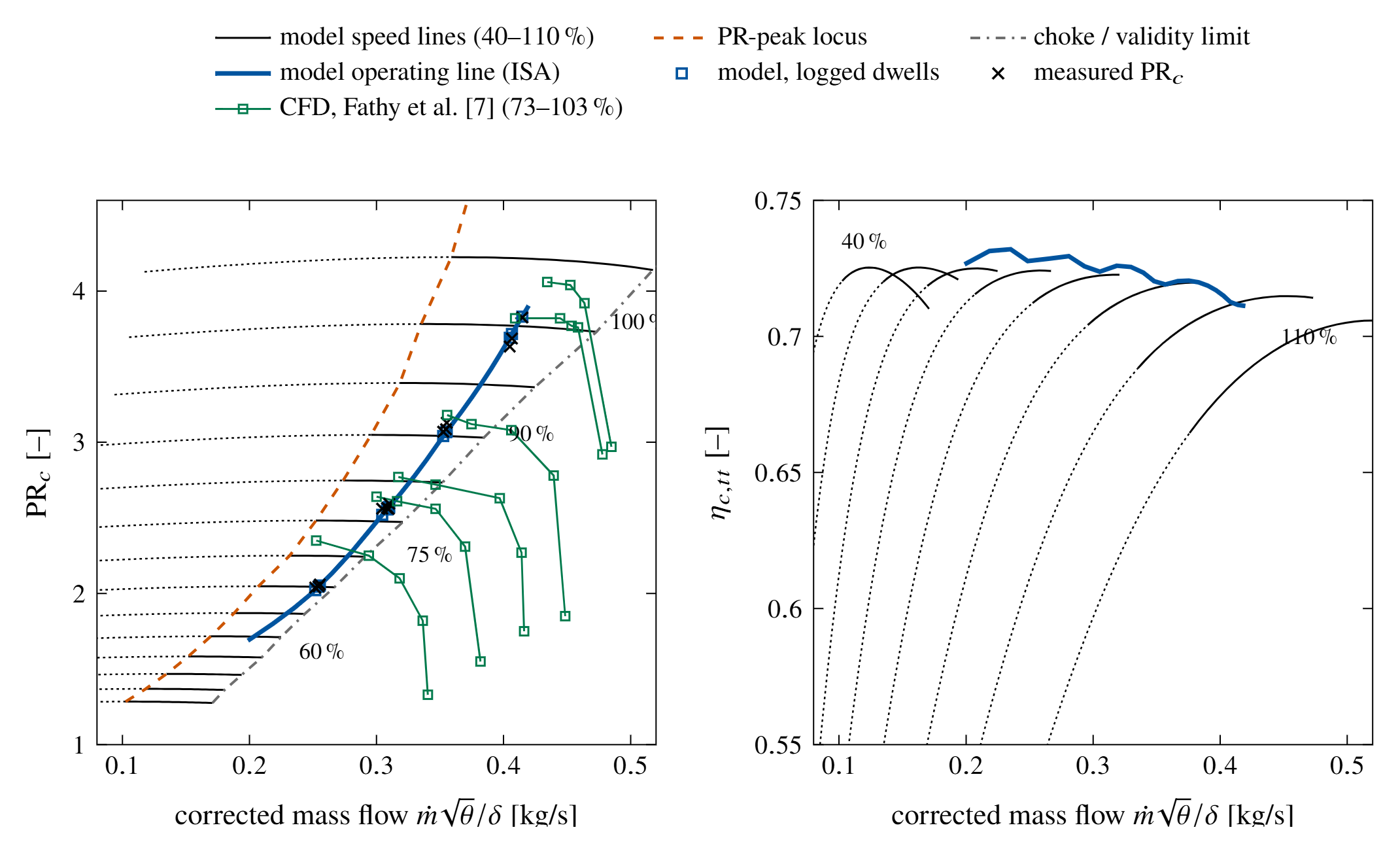
The compressor map comes from a mean-line model of the impeller and the vaned diffuser. The model uses the scanned P200-SX geometry (\(D_2=84\) mm, 6+6 blades, 17-vane diffuser) [1]. An optimum set of internal and parasitic losses closes the Euler work with slip. I calibrate only two scalars: \(\psi_{\mathrm{res}}=0.0681\) and \(K_d=0.345\). I invert the map on its stable branch only, and I reject positive-slope solutions instead of clipping them.
Compressor efficiency from the Euler work \(\Delta h_E\) and the loss terms. Turbine flow is a choked capacity with an ellipse-law reduction below \(\mathrm{PR}_{\mathrm{crit}}=1.7\). A separate mean-line turbine model, calibrated only at full speed, reproduces the identified part-speed efficiency trend within 0.0056.
Two lumped thermal nodes store heat in the compressor casing and the hot section. Observation models translate the gas states into what the rig actually reads:
- sheathed T3 and T4 thermocouples, with convection, radiation and lag
- a nozzle-exit pitot, with friction loss.
The sensor dynamics stay separate from the engine physics.
HowThe Simulink model
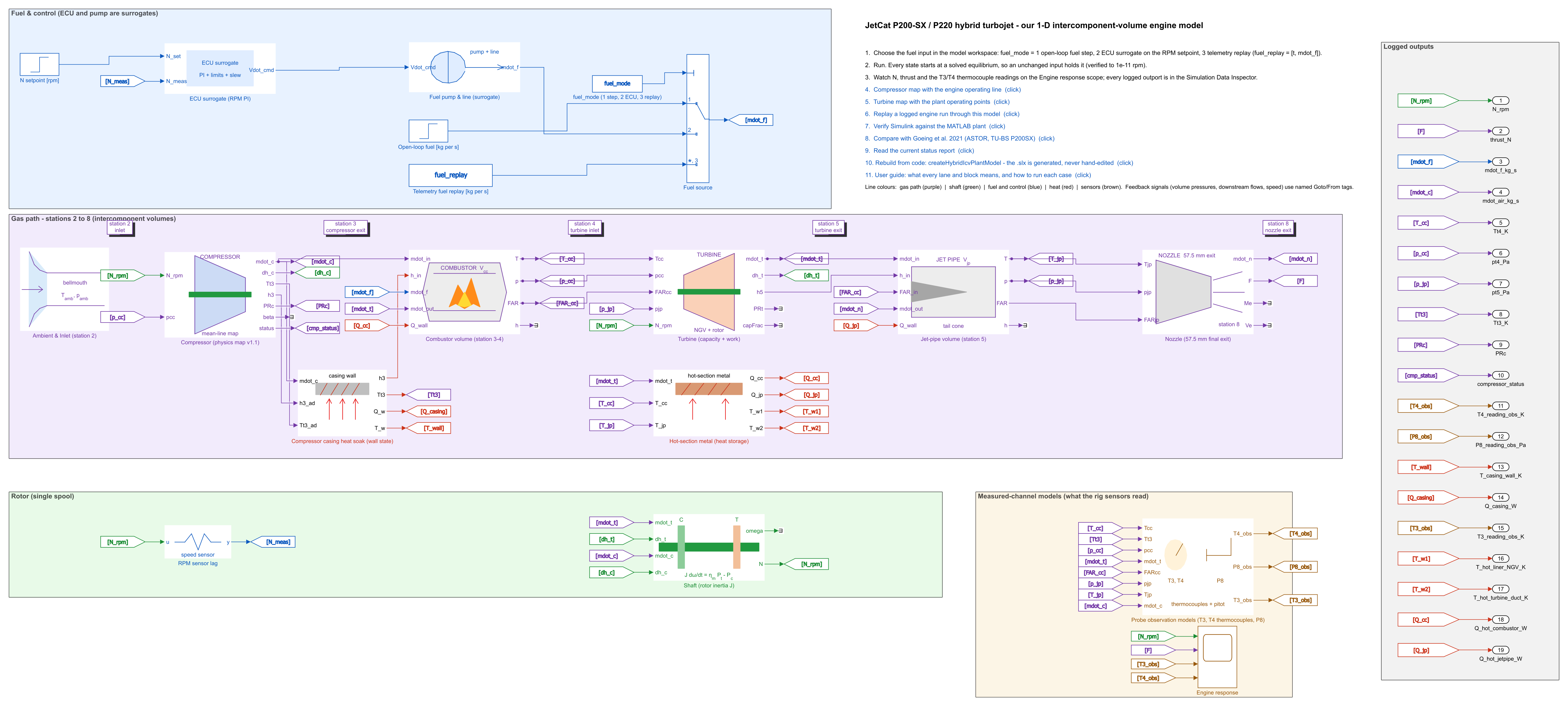
A script generates the Simulink model from the same component kernels as the MATLAB plant. Each kernel is a MATLAB Function block in a masked subsystem. The forward gas-path signals run left to right, and the feedback signals use named tags.
There are three selectable fuel inputs:
- an open-loop step
- a PI speed governor that stands in for the ECU (a surrogate, not identified)
- replay of a logged fuel history.
Every state starts at a solved equilibrium, which holds to \(10^{-11}\) rpm with an unchanged input.

HowCalibration kept apart from assessment
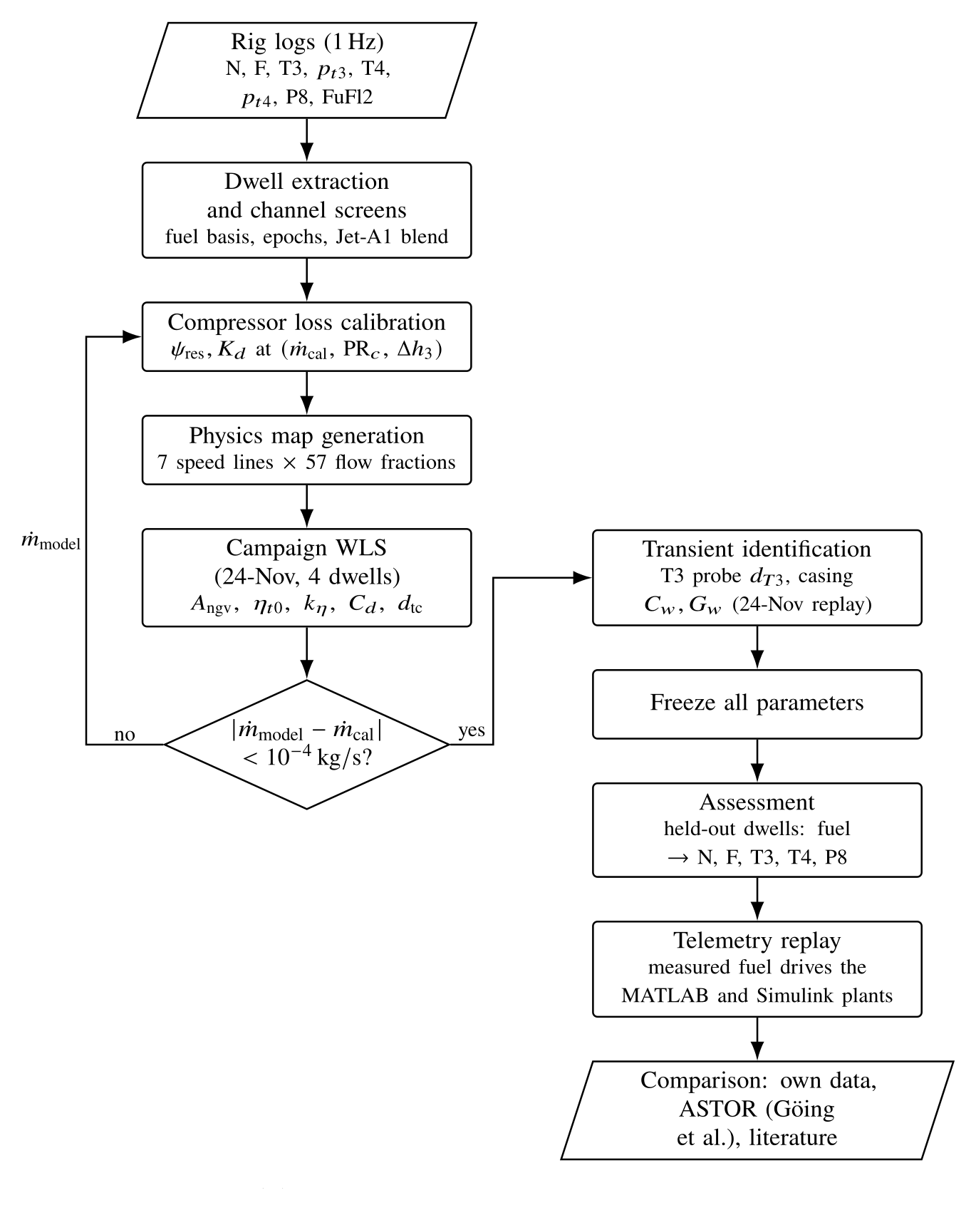
I identified the global parameters by weighted least squares on a single four-dwell campaign. These are the NGV area, the turbine efficiency and its speed slope, the nozzle effective area, and the thermocouple diameter. The transient parameters (T3 probe and casing node) came from a replay of that same run. Then I froze all parameters.
The compressor calibration is self-consistent. It uses the air flow that the model itself predicts at the 100% dwell (0.413 kg/s). I iterated it until that flow changed by less than \(10^{-4}\) kg/s [1].
The assessment uses only held-out data. These are Jet A runs from November 2025 and March 2026, with dwells at 70, 80, 90 and 100% speed (78 to 112 krpm).
HowWhat drives a replay
The measured fuel flow is the only time-varying input of a replay. It is not the only information that enters [1]:
- the ambient temperature and pressure of the run
- the configuration: the P200-SX core, the P220 nozzle and the parameters frozen on the calibration campaign
- the initial condition: each segment starts from a solved equilibrium at its first fuel sample. After that, the model is never reset to the measurements.
ResultsSteady dwells: speed and thrust from fuel flow
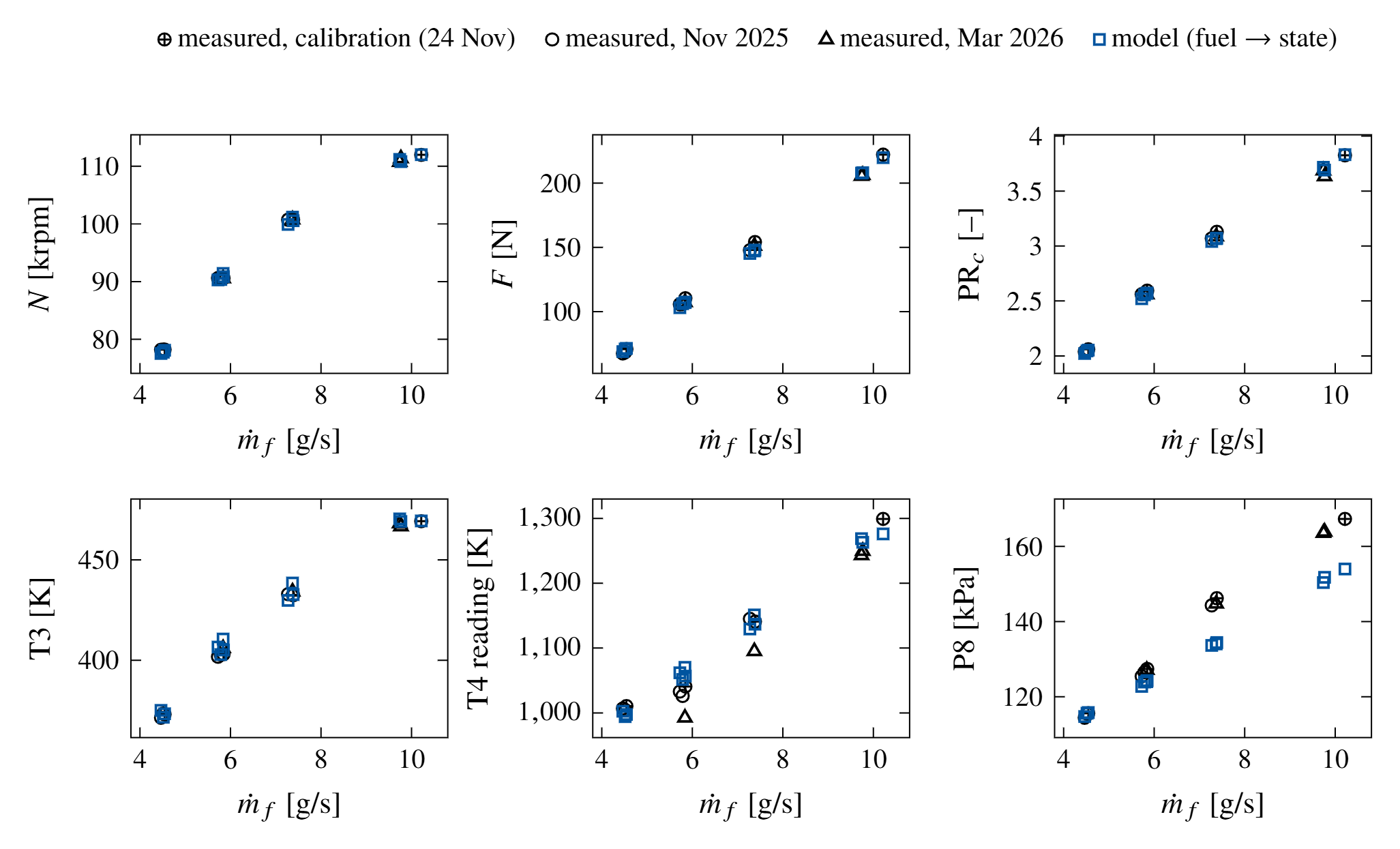
I solved each of the 9 held-out Jet A dwells from its measured fuel flow, with all parameters frozen. The errors differ by channel [1]:
- shaft speed: 0.61% RMS (maximum 0.96%)
- thrust: 2.0% RMS (2.3 N)
- turbine-inlet pressure: within 0.9%
- T3 reading: 1.9 K mean error
- T4 reading: 19 K RMS on the November runs, but 43 K too high on average on the March runs
- P8 reading: not reproduced at high power (see below).
On the March runs, speed, thrust and pressures still agree. I therefore attribute the T4 offset to a shift of the T4 channel itself.
ResultsFull-run replays: two error measures
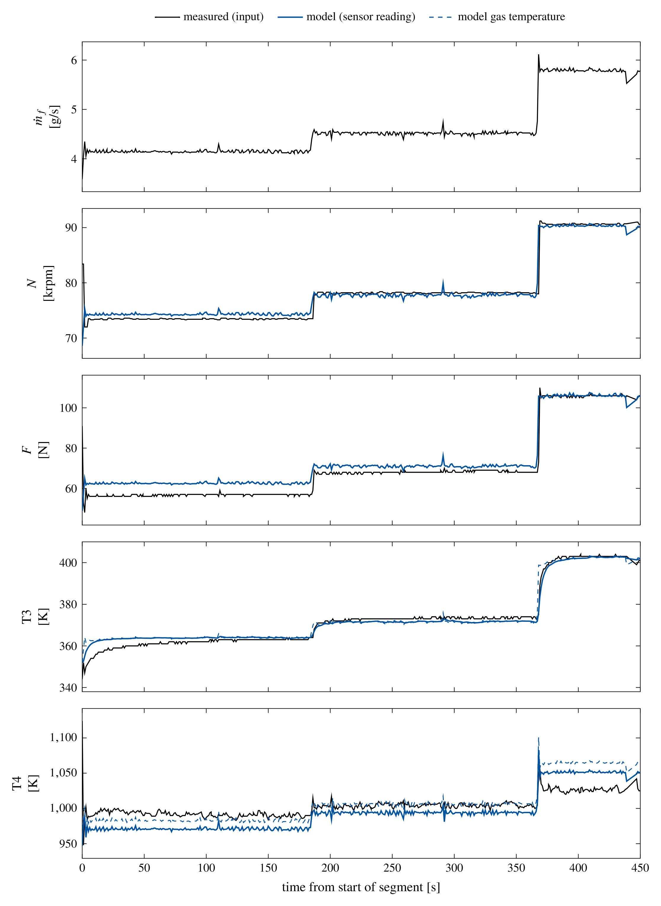
I replayed seven complete Jet A runs: six held out and the calibration run. I report two error measures, because they answer different questions [1]:
- Quasi-steady samples isolate the plant. The RMS errors are 0.45–0.97% in speed and 1.1–4.0 N in thrust.
- Complete segments also include the one-to-two-second throttle ramps of the engine control unit. The 1 Hz log resolves these ramps poorly. The RMS errors are 0.88–3.97% in speed and 4.1–8.4 N in thrust.
On quasi-steady samples, the T3 reading follows within 1.9–6.1 K RMS. The T4 error is 18–20 K on the November runs. On the March runs it is 18–76 K, mostly as a constant offset.
The model follows the throttle steps in speed, thrust and T3 without a reset. It does not reproduce every channel equally well. The Simulink implementation matches the MATLAB plant to within half a revolution per minute in the same replay.
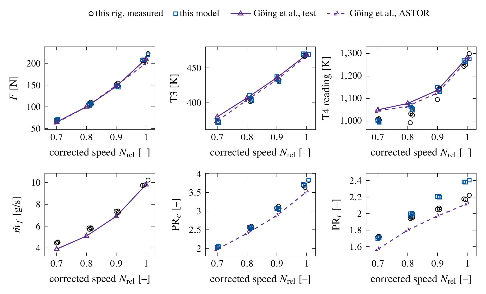
I also compared the model with the ASTOR model and test data of Göing et al. for a second, deteriorated P200-SX [2]. With a fuel ramp read from their fuel trace, the model reaches 95% of the 70–100% speed step in 2.36 s. The measured time is 2.0 s. The spool-up time depends strongly on that assumed ramp [1].
The compressor-exit temperature needed one more step. I separated the thermocouple lag from the casing heat soak. The model then gave a T3 rise of 7.2 K during the 100% dwell, against 8 K measured [1].
LimitsThe air flow is inferred
The model gives an air mass flow at every instant, but the rig has no air-flow measurement. The estimate is therefore model-dependent, and nothing validates it directly [1].
Two parts of the method set its level:
- Without a bellmouth, the air flow follows from the identified turbine capacity area and nozzle coefficient.
- Near design, the compressor speed line is flat. The assumed combustion efficiency and the T4 reading therefore set most of the air-flow level.
A bellmouth measurement would fix that level. The rotor inertia and the hot-section thermal nodes are also not identifiable from 1 Hz logs. The inertia comes from the CAD shaft model of Göing et al. The hot-section nodes come from part masses, areas and heat-transfer estimates. The model omits gas momentum, so it does not apply to surge or rotating stall.
LimitsThe nozzle-exit pitot (P8) discrepancy
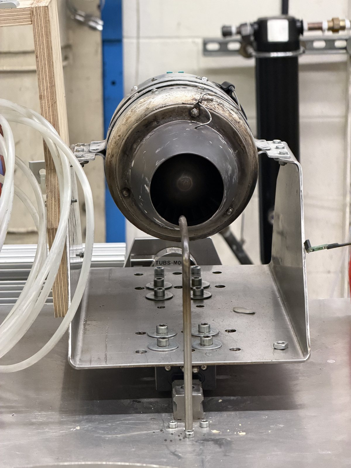
P8 is the one channel the model does not reproduce across the power range. The model is close to the reading at 78 krpm and about 3 kPa low at 90.6 krpm. At 100.7–112 krpm it is 10–13 kPa low, in every campaign [1].
Suppose P8 is the total pressure of a uniform jet. Then the measured thrust and P8 imply an air flow 7–9% below the model at 90–100% speed. That inversion also needs a combustion efficiency that falls from 0.93 to about 0.86. No constant parameter produces this change.
Three single-cause explanations remain:
- The true air flow is lower than the model at high power. In that case, the model over-predicts the air flow there.
- The thrust stand reads low above about 150 N.
- The single P8 probe does not represent the mass-averaged jet total pressure at high power.
Fig. 6 shows why the third explanation is plausible. The pitot probe with its embedded thermocouple is the only Station 8 measurement, and it is not on the jet centerline.
The steady data cannot separate the first and third explanations. A P8 traverse, a dead-weight thrust calibration to 250 N and a bellmouth wall-static tap would separate them. P8 does not steer the identified parameters. The speed, thrust and temperature predictions therefore do not depend on the answer [1].
ResultsA data issue the model found
The model explained an apparent instrument epoch as a change in the fuel-flow measurement basis. Until November 2025, the flowmeter also measured the bearing-lubrication bypass, about 0.76 g/s [1].
References
- [1]S. Sharma, “A physics-based intercomponent-volume model of a micro-turbojet: model-generated component maps, thermal storage and sensor models, validated against JetCat P200-SX test-cell data,” manuscript in preparation, October 2026.
- [2]J. Göing et al., ASTOR (Aircraft Engine Simulation for Transient Operation Research) model and P200SX transient test data, TU Braunschweig, 2021. Full references to the compressor geometry (Fathy et al.), the mean-line loss set (Oh et al.) and the NASA polynomials are in [1].