Euler-JEPA
Numerical learning exerciseCan a world model learn the dynamics of a rotor only by listening to it? I built a JEPA world model that learns from unlabeled sound and plans control actions in its own latent space. It needs very few labels and it tolerates acoustic noise. A physics pipeline that knows the true equation is still more accurate when the sensor is clean.
WhyWhy version 1 could not work
Version 1 of this project was an honest audit with a negative result. When I read the code again, I found that the result came from the setup of the study.
- The model saw the rotor speed directly and without noise, so representation learning had nothing to do.
- The latent prediction was only a small extra loss. A separate head made the forecast, so the JEPA objective could not improve it.
- The control input was constant in each sequence. No model could therefore learn how the speed responds to a control change.
- The equilibrium speed was near 21 rad/s, but every sequence started near 400 rad/s. Each sequence was therefore only a spin-down.
I also use this rotor as a toy test for my turbulence work. Before I consider JEPA for recovering unresolved turbulence, I want to see it work on a problem where every answer is known.
WhatA rotor you can only hear
Version 2 keeps the physics but asks the question that JEPA is designed for. Euler turbomachinery work drives the rotor, and an actuator with lag and delay sets the swirl. Each episode has six hidden parameters, and the commands change all the time.
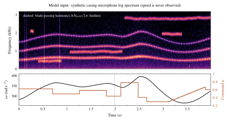
Rotor balance from Euler work with a lagged, delayed actuator. \(\dot m, J, k_\omega, c_2, \tau_a, d\) change in each episode, and the models never see them.
The models never see the speed. Every 10 ms they see a 64-bin spectrum of a synthetic casing microphone. It contains blade-passing tones, flow noise, distractor tones from other machines, bursts and gain drift.
HowLearning in representation space
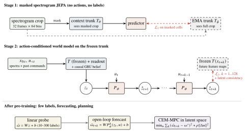
Stage 1 learns spectrogram features by masked latent prediction, with no labels and no actions. Stage 2 freezes those features. Then an action-conditioned predictor learns to forecast the future features in latent space.
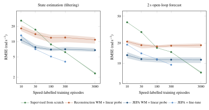
A small probe reads the speed from the latent with 10 to 300 labeled episodes. The same model forecasts the speed and plans control actions with model predictive control. I compared it with a reconstruction world model, supervised training and a classical pipeline. That pipeline gets the true equation of motion, which the learned models do not get.
ResultsWhat I found
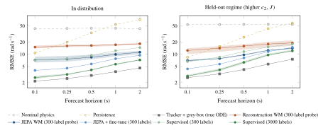
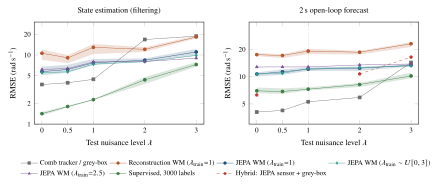
The JEPA model also learned how the speed responds to a control change. The median error of the 2 s control gain is 10 %. In version 1, the learned models did not respond to the control at all.
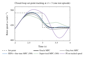
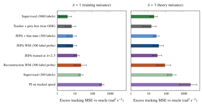
Planning directly in the JEPA latent tracks the set-points almost as well as an oracle that knows the true state. This is the part that is very interesting to me, and very cool. A controller that learned only from sound plans almost as well as a physics model that gets the equation.
LimitsWhere it does not win
The physics pipeline is still more accurate in distribution: 4.6 rad/s against 11.3 rad/s for the 2 s forecast. The latent recovers the speed well, but it recovers the hidden machine parameters only partly. It almost does not find the inertia or the delay, so long forecasts drift.
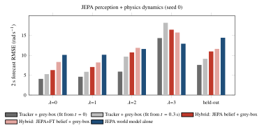
I tested four more ideas. Longer training rollouts gave the largest single gain. Training on random noise levels made the speed estimate much better under noise, but the forecasts did not follow. A seed ensemble reduced the error by 9 %, but its uncertainty was overconfident.
LessonsWhat broke along the way
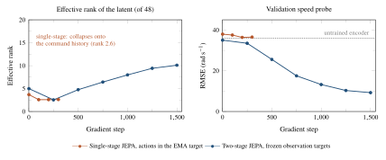
Like the Sandia work, this runs on my gaming laptop. The hardware and its limits are on the Sandia Flame D page. The 4 GB GPU kept every model small, and the GPU is shared with other jobs on the same machine.