Schlieren Visualization of Natural Convection

The bench in the dark lab: an 8 ft focal-length concave mirror, the light source and a candle in the test section

Optical layout: a 3 mm pinhole source and two concave mirrors in a Z-fold, with the test section between them and a razor-blade knife edge before the camera

The four test configurations: a horizontal plate and a 25.5° plate, each at the low (360 °C) and high (570 °C) settings

Schlieren Visualization of Natural Convection

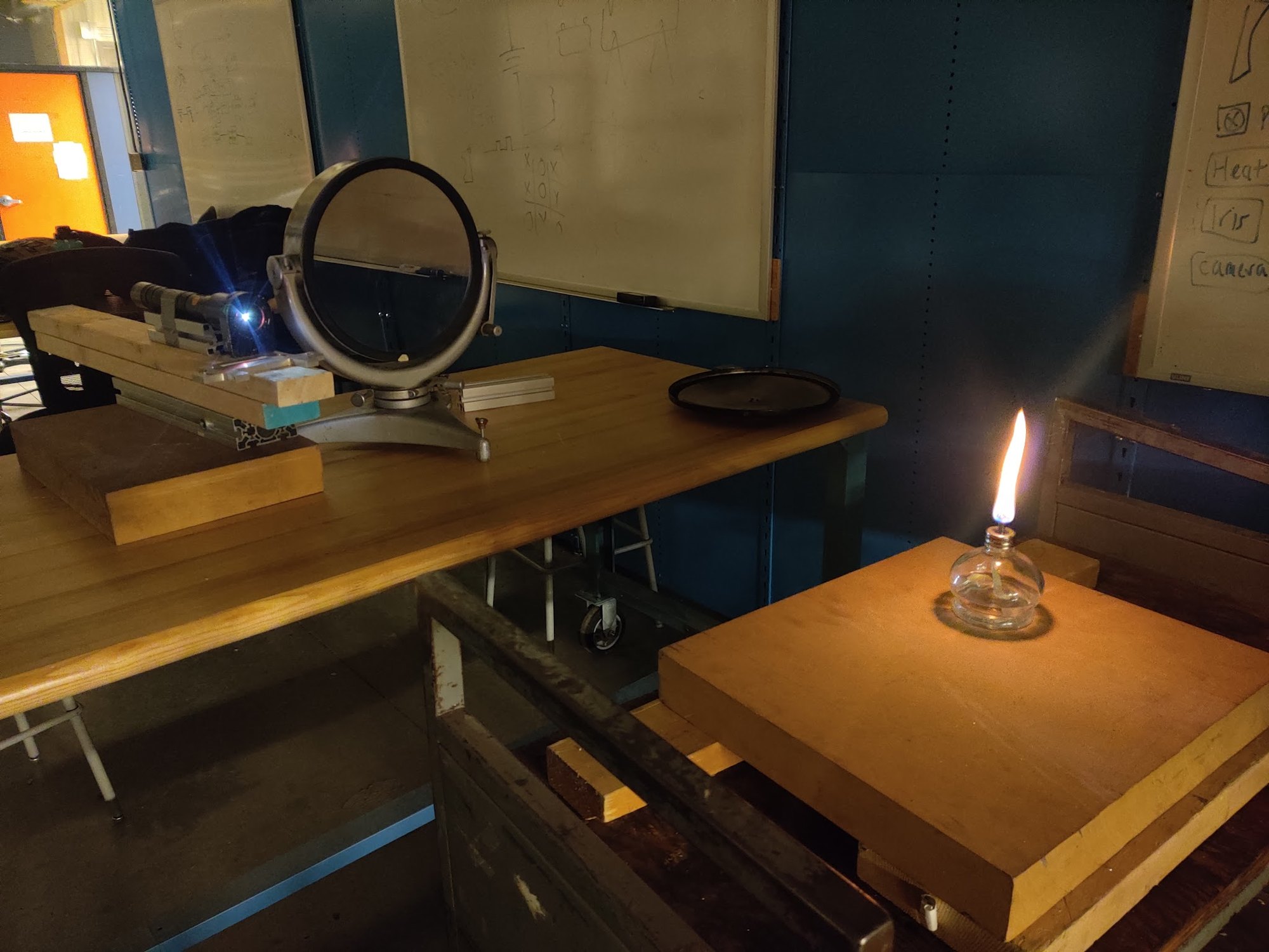
Course project

A group lab in MECH 489, an undergraduate experimental thermofluids course. We built a two-mirror schlieren system from a flashlight, a drilled aluminum block, two 8-foot mirrors and a razor blade. We used it to watch hot air rise off a heated plate at two temperatures and two angles. The result is mainly qualitative: it shows how the flow changes.

Result

Clear visualizations of the flow. At the higher temperature the plume is turbulent throughout. On the tilted plate, a laminar layer near the lower edge breaks into eddies higher up. An exploratory speed estimate gave apparent feature speeds of roughly 30–170 mm/s. These are not validated fluid velocities.

My part

Steve Rogak suggested that we try to extract velocity information. Within Group 2, I did that quantitative part: the image-processing scripts and the feature-speed estimates.

Team

Group 2: Sid Sharma, Matt McEachern, Drew Setoguchi and Connor Block (MECH 489, January–February 2025)

Methods & tools

Z-type two-mirror schlieren · DSLR video · MATLAB image processing (wavelet denoising, Fourier streak filtering, median background) · feature tracking · t-based confidence intervals

Links

Results deck

Project breakdown

WhatMaking invisible air visible

Air that rises off a hot surface is invisible, but it is not uniform. Hotter air is less dense and bends light slightly differently. Schlieren imaging turns that small bending into brightness. As a result, plumes, laminar sheets and turbulent eddies show on camera without any seeding [2, 3].

The lab asked two questions: how does the flow change as the plate gets hotter, and what happens when the plate is tilted?

Buoyancy drives the flow. Air near the plate heats, expands, becomes lighter than the air around it and rises. The Rayleigh number compares the buoyant forcing with the viscous and thermal damping. It indicates whether the air rises smoothly or breaks into eddies:

\[\rho\approx\rho_0\big[1-\beta\,(T-T_0)\big],\qquad \mathrm{Ra}_L=\mathrm{Gr}_L\,\mathrm{Pr}=\frac{g\,\beta\,(T_s-T_\infty)\,L^3}{\nu^2}\,\mathrm{Pr}\]

The Boussinesq density relation with the thermal expansion coefficient \(\beta\), and the Rayleigh number for a plate of length \(L\) at surface temperature \(T_s\). At low \(\mathrm{Ra}_L\) the flow stays laminar. At higher \(\mathrm{Ra}_L\) it becomes turbulent.

This picture is only qualitative here. The Boussinesq form assumes small density changes, \(\beta\,(T_s-T_\infty)\ll1\). For air, \(\beta\approx1/T_\infty\). With room air near 20 °C, the plate at 360 °C or 570 °C is about two to three times the room temperature in kelvin. The density near the plate changes by a large factor, so the Rayleigh number is an order-of-magnitude guide only.

HowA schlieren system from a flashlight and a razor blade

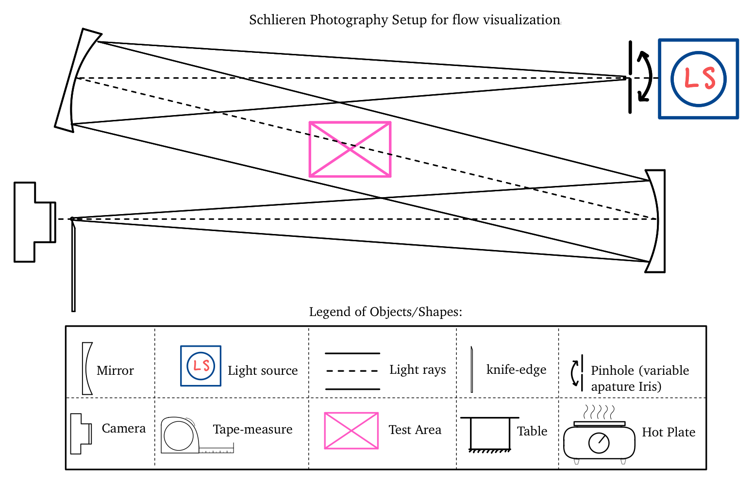
A 7000-lumen LED flashlight shines through a 3 mm hole drilled in an aluminum block. This makes a near point source. The source is one focal length (8 ft) from the first concave mirror. That mirror sends a collimated beam across the test section to the second mirror. The second mirror focuses the beam onto a razor blade that covers half the image of the source. A DSLR is directly behind the blade.

A density gradient in the test section bends a ray, so the ray lands slightly off the focus. The razor blade then blocks more or less of that ray, and the gradient shows as a light or dark band on the camera:

\[n-1=K\rho,\qquad \varepsilon_y=\frac{1}{n_0}\int\frac{\partial n}{\partial y}\,dz,\qquad \frac{\Delta I}{I}\propto\frac{f_2\,\varepsilon_y}{a}\]

The Gladstone–Dale relation links refractive index to density. The ray deflection \(\varepsilon_y\) integrates the index gradient along the beam. The knife edge turns this deflection into a contrast change. The contrast change increases with the mirror focal length \(f_2\) and decreases with the unobstructed source height \(a\).

Video 1 — Our alignment check: the heat that rises off a hand shows above the fingers. This confirmed the optical sensitivity before the hot plate went in. It says nothing about velocity accuracy.

Getting it to work was mostly patience. The knife-edge position, the focal distances, the mirror heights and even drafts in the room all changed the image. Our check was simple: if the heat off a hand shows, the system is sensitive enough to see the plate.

ResultsWhat the flow did

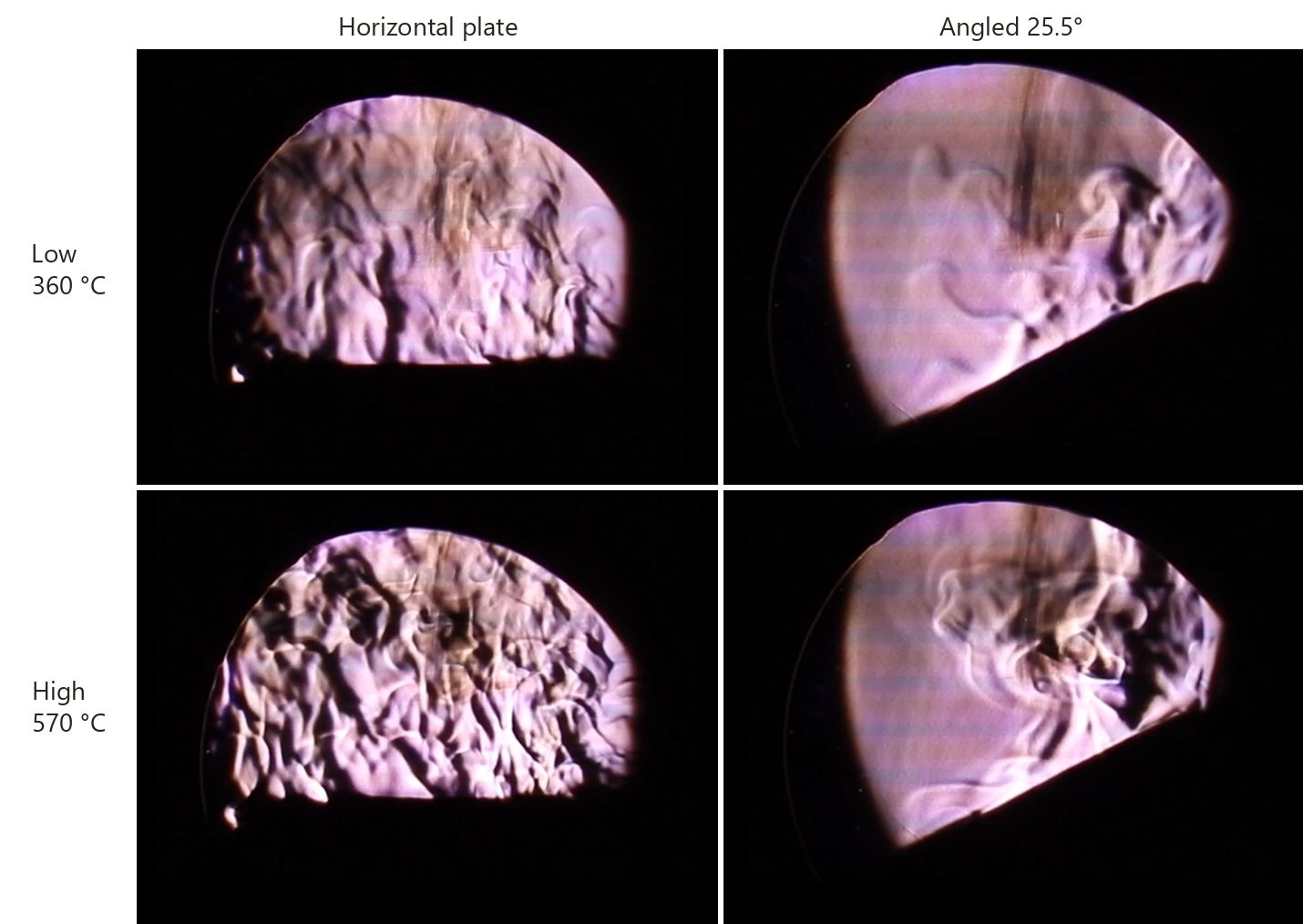
Video 2 — The four configurations side by side, in the same layout as the Result view at the top. It shows low (top) and high (bottom) temperature, and horizontal (left) and 25.5° plate (right).

Temperature drives transition. At the low setting (surface ≈ 360 °C), the flow is a mix of laminar sheets and turbulent pockets. At the high setting (≈ 570 °C), it is turbulent throughout. The contrast is also much stronger, because the density difference is larger.
Tilting the plate organizes the flow. Over the 25.5° plate, air runs up the surface as a smooth laminar layer near the lower edge. Near the top, it breaks into vertical turbulent eddies. This happens at both temperatures and is stronger at the high setting.

Video 3 — The angled plate after a deliberate disturbance: the plume falls over and forms again along the surface in about three seconds.

HowAn exploratory step: apparent feature speeds

The lab was mainly qualitative. Steve Rogak suggested that we also try to get velocity information from the videos. I wrote MATLAB scripts that clean each video and track the moving structures:

The scripts subtract a 50-frame median image as the background (tare).
Fourier-domain filtering removes the horizontal streaks that the camera adds.
Optional wavelet denoising and Gaussian smoothing suppress speckle.
The scripts then detect bright features and track their centroids between frames.

I made five processing variants (six for one case), with different filtering, smoothing and blending choices [1, 4, 5]. A group member also made three manual estimates per case. These used a ruler on screen, with the plate diameter as the scale.

\[u=\frac{\Delta x_{\mathrm{px}}\,s}{\Delta t},\qquad \bar u\pm t_{0.975,\,n-1}\,\frac{s_u}{\sqrt n}\]

Feature displacement in pixels, scaled by the image scale \(s\) (from the known plate diameter), over the frame interval \(\Delta t\). The second term is the mean of the \(n\) pooled estimates, with a t-based 95% interval.

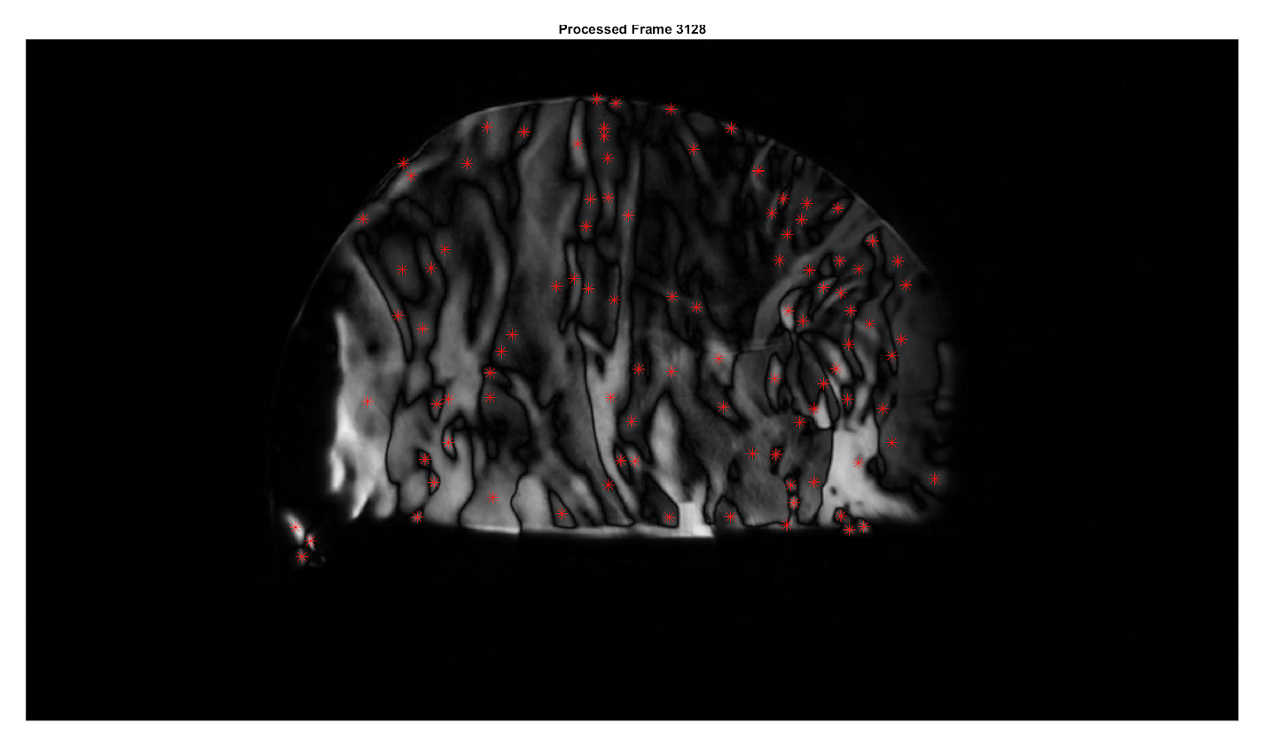
Fig. 1 — A processed frame from the high-temperature horizontal case, with the background removed, the streaks filtered and the tracked features marked in red.

What a tracked feature measures is the apparent speed of a refractive-index pattern in the image. It is not a validated fluid velocity. The pattern speed depends on the processing, the feature detection and the image scale.

Apparent feature speeds, pooled over the script variants and manual estimates for one video per case [1]
Case	Pooled mean	t-based 95% interval	SDOM
Horizontal, low	32.7 mm/s	14.0–51.3	7.9 mm/s
Horizontal, high	109.9 mm/s	62.3–157.6	20.7 mm/s
Angled 25.5°, low	99.7 mm/s	44.9–154.5	23.2 mm/s
Angled 25.5°, high	165.7 mm/s	98.0–233.3	28.6 mm/s

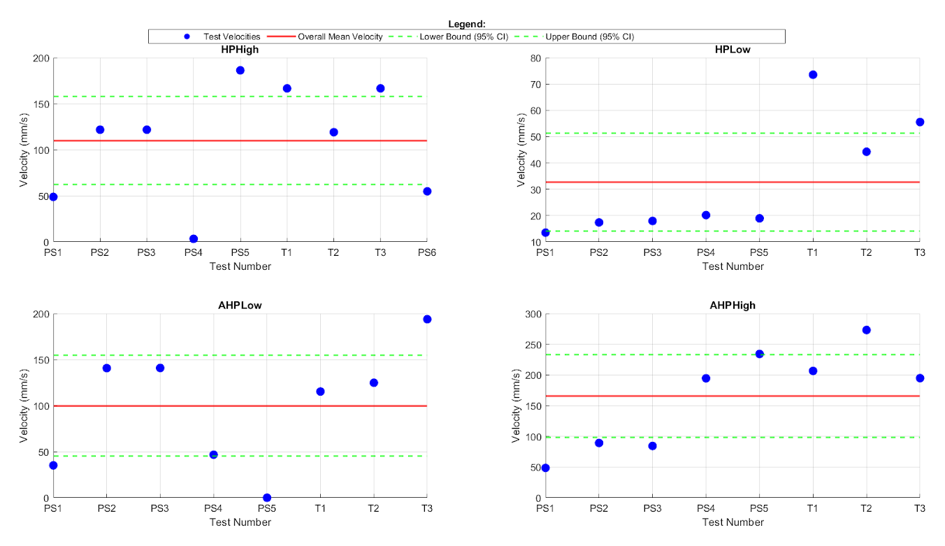
Fig. 2 — Speed estimates for each case from the script variants (PS) and the manual estimates (T). Red is the pooled mean and green the t-based 95% bounds.

Read the intervals with care. Each interval comes from 8 or 9 estimates of the same video. The estimates come from alternative processing methods and manual readings of the same recordings. The interval therefore describes the spread between methods.

The methods also disagree in a systematic way. In the horizontal low case, every script estimate is below 21 mm/s and every manual estimate is above 40 mm/s. In the angled low case, one script variant recorded no features and enters the pool as zero.

Within those limits, one ordering is clear. For the horizontal plate, the high setting gives faster apparent features than the low setting, and the intervals do not overlap. The other comparisons have overlapping intervals, so this data cannot resolve them.

The results deck from this project also states that Monte Carlo simulations validated turbulence-intensity measurements. I do not repeat that claim here, because the lab report contains no analysis that supports it.

Looking back, the fixes are clear:

a scale target of known size in the frame
thermocouples to record the true surface temperature
repeat recordings of each case, to separate run-to-run variation from processing choices
an independent velocity reference, to test whether the pattern speeds track the air
a dual knife edge for contrast.

The same idea, measuring flow from how a background appears to move, is what I later took to a phone camera in BOScope.

References

[1]S. Sharma, M. McEachern, D. Setoguchi and C. Block, “Experiment 1: Heat transfer and flow pattern in natural convection,” MECH 489 lab report (Group 2), University of British Columbia, Feb. 2025.
[2]G. S. Settles, Schlieren and Shadowgraph Techniques: Visualizing Phenomena in Transparent Media, Springer, 2001.
[3]B. Atcheson, “Schlieren-based flow imaging,” M.Sc. thesis, University of British Columbia, 2007.
[4]Q. Wang, Y. Wu, H. T. Cheng, X. H. Mei and C. Y. Zhao, “A schlieren motion estimation method for seedless velocimetry measurement,” Exp. Therm. Fluid Sci. 109, 109880, 2019.
[5]H. Nobach and M. Honkanen, “Two-dimensional Gaussian regression for sub-pixel displacement estimation in particle image velocimetry or particle position estimation in particle tracking velocimetry,” Exp. Fluids 38, 511–515, 2005.